library(tidyverse)
library(gov50data)
library(gapminder)Gov 50 Cheat Sheet
R Basics (Week 1)
Creating a vector
You can create a vector using the c function:
## Any R code that begins with the # character is a comment
## Comments are ignored by R

my_numbers <- c(4, 8, 15, 16, 23, 42) # Anything after # is also a
# comment
my_numbers
[1] 4 8 15 16 23 42Installing and loading a package
You can install a package with the install.packages function, passing the name of the package to be installed as a string (that is, in quotes):
install.packages("ggplot2")You can load a package into the R environment by calling library() with the name of package without quotes. You should only have one package per library call.
library(ggplot2)Calling functions from specific packages
We can also use the mypackage:: prefix to access package functions without loading:
knitr::kable(head(mtcars))| mpg | cyl | disp | hp | drat | wt | qsec | vs | am | gear | carb | |
|---|---|---|---|---|---|---|---|---|---|---|---|
| Mazda RX4 | 21.0 | 6 | 160 | 110 | 3.90 | 2.620 | 16.46 | 0 | 1 | 4 | 4 |
| Mazda RX4 Wag | 21.0 | 6 | 160 | 110 | 3.90 | 2.875 | 17.02 | 0 | 1 | 4 | 4 |
| Datsun 710 | 22.8 | 4 | 108 | 93 | 3.85 | 2.320 | 18.61 | 1 | 1 | 4 | 1 |
| Hornet 4 Drive | 21.4 | 6 | 258 | 110 | 3.08 | 3.215 | 19.44 | 1 | 0 | 3 | 1 |
| Hornet Sportabout | 18.7 | 8 | 360 | 175 | 3.15 | 3.440 | 17.02 | 0 | 0 | 3 | 2 |
| Valiant | 18.1 | 6 | 225 | 105 | 2.76 | 3.460 | 20.22 | 1 | 0 | 3 | 1 |
Data Visualization (Week 2)
Scatter plot
You can produce a scatter plot with using the x and y aesthetics along with the geom_point() function.
ggplot(data = midwest,
       mapping = aes(x = popdensity,
                     y = percbelowpoverty)) +
  geom_point()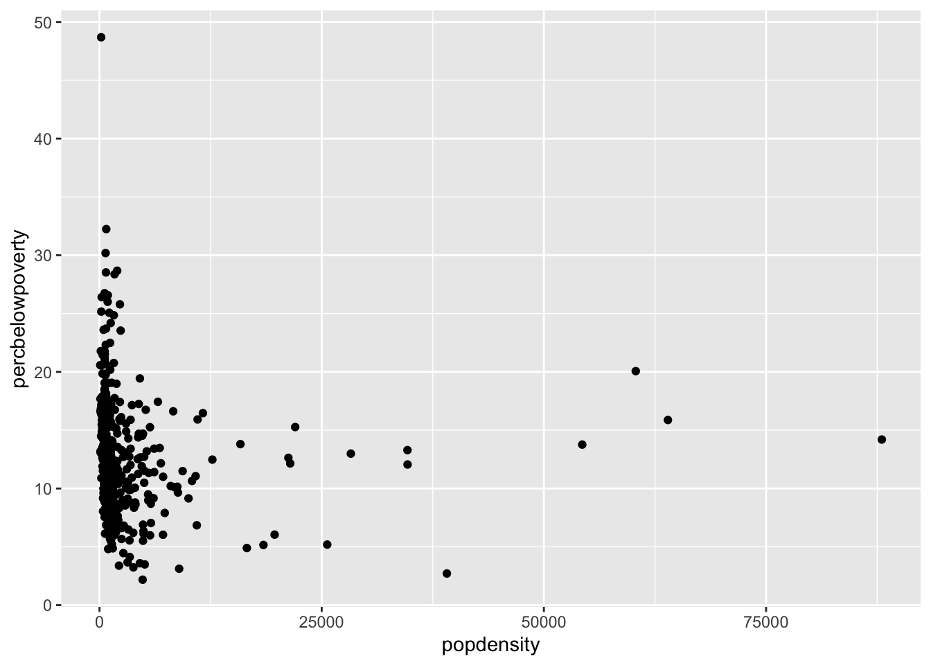
Smoothed curves
You can add a smoothed curve that summarizes the relationship between two variables with the geom_smooth() function. By default, it uses a loess smoother to estimated the conditional mean of the y-axis variable as a function of the x-axis variable.
ggplot(data = midwest,
       mapping = aes(x = popdensity,
                     y = percbelowpoverty)) +
  geom_point() + geom_smooth()
`geom_smooth()` using method = 'loess' and formula = 'y ~ x'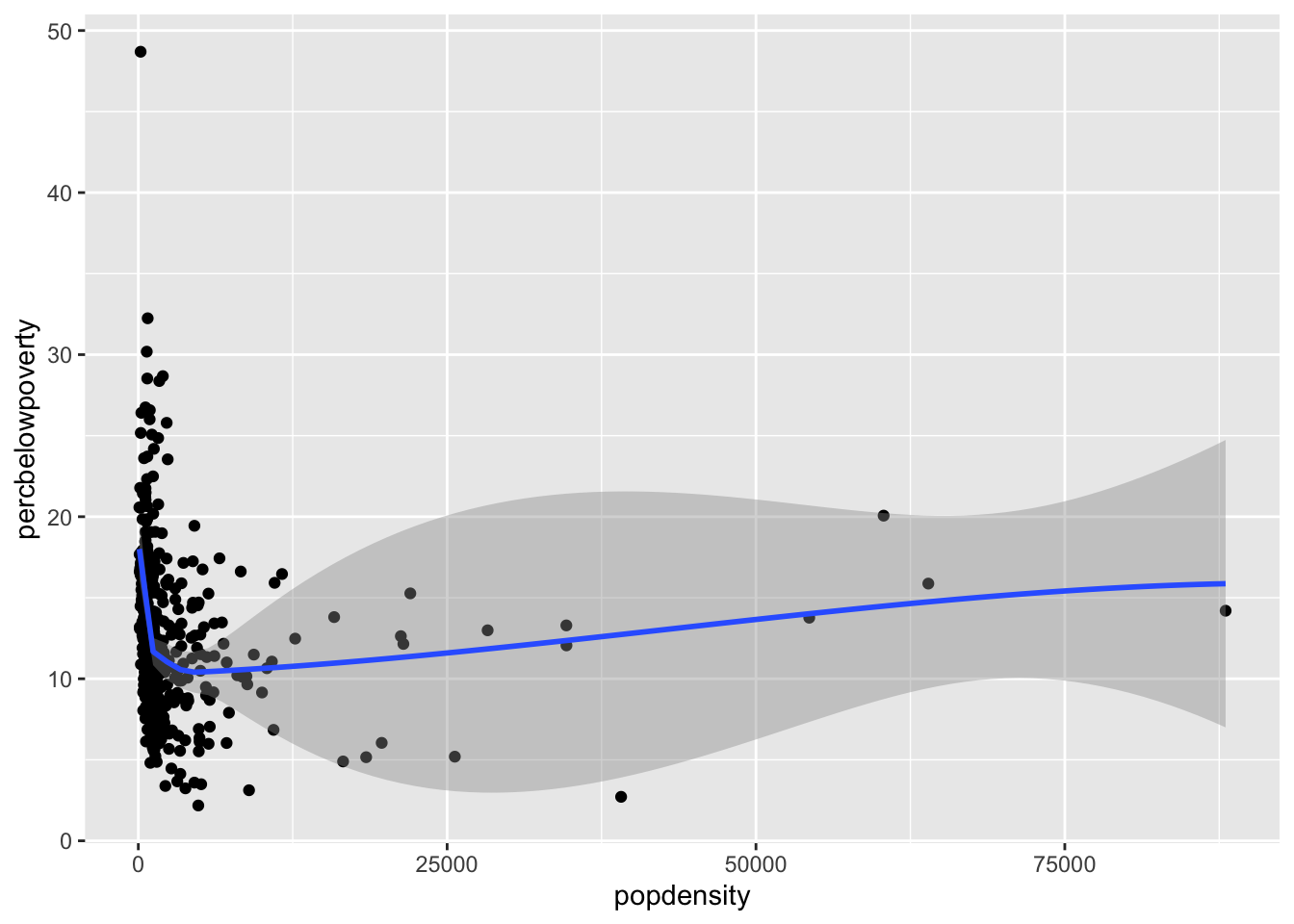
Adding a regression line
geom_smooth can also add a regression line by setting the argument method = "lm" and we can turn off the shaded regions around the line with se = FALSE
ggplot(data = midwest,
       mapping = aes(x = popdensity,
                     y = percbelowpoverty)) +
  geom_point() + geom_smooth(method = "lm", se = FALSE)
`geom_smooth()` using formula = 'y ~ x'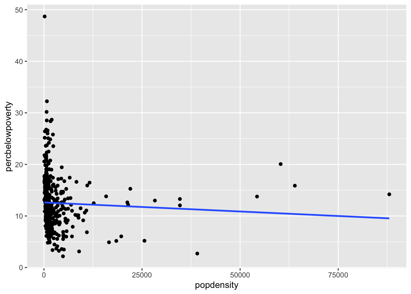
Changing the scale of the axes
If we want the scale of the x-axis to be logged to stretch out the data we can use the scale_x_log10():
ggplot(data = midwest,
       mapping = aes(x = popdensity,
                     y = percbelowpoverty)) +
  geom_point() +
  geom_smooth(method = "lm", se = FALSE) +
  scale_x_log10()
`geom_smooth()` using formula = 'y ~ x'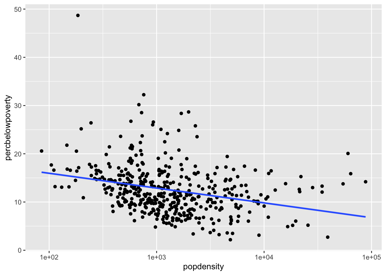
Adding informative labels to a plot
Use the labs() to add informative labels to the plot:
ggplot(data = midwest,
       mapping = aes(x = popdensity,
                     y = percbelowpoverty)) +
  geom_point() +
  geom_smooth(method = "loess", se = FALSE) +
  scale_x_log10() +
  labs(x = "Population Density",
       y = "Percent of County Below Poverty Line",
       title = "Poverty and Population Density",
       subtitle = "Among Counties in the Midwest",
       source = "US Census, 2000")
`geom_smooth()` using formula = 'y ~ x'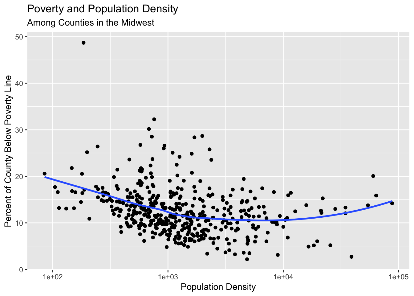
Mapping aesthetics to variables
If you would like to map an aesthetic to a variable for all geoms in the plot, you can put it in the aes call in the ggplot() function:
ggplot(data = midwest,
       mapping = aes(x = popdensity,
                     y = percbelowpoverty,
                     color = state,
                     fill = state)) +
  geom_point() +
  geom_smooth() +
  scale_x_log10()
`geom_smooth()` using method = 'loess' and formula = 'y ~ x'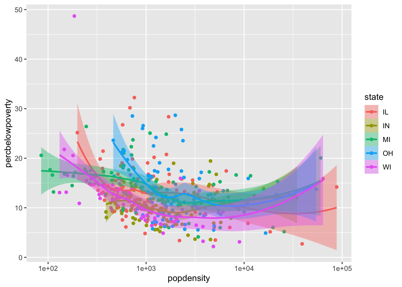
Mapping aesthetics for a single geom
You can also map aesthetics for a specific geom using the mapping argument to that function:
ggplot(data = midwest,
       mapping = aes(x = popdensity,
                     y = percbelowpoverty)) +
  geom_point(mapping = aes(color = state)) +
  geom_smooth(color = "black") +
  scale_x_log10()
`geom_smooth()` using method = 'loess' and formula = 'y ~ x'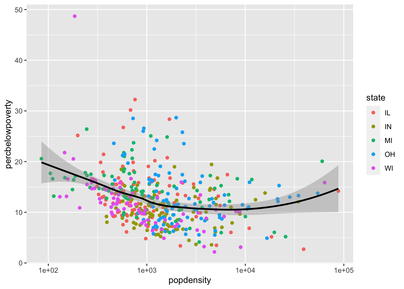
Setting the aesthetics for all observations
If you would like to set the color or size or shape of a geom for all data points (that is, not mapped to any variables), be sure to set these outside of aes():
ggplot(data = midwest,
       mapping = aes(x = popdensity,
                     y = percbelowpoverty)) +
  geom_point(color = "purple") +
  geom_smooth() +
  scale_x_log10()
`geom_smooth()` using method = 'loess' and formula = 'y ~ x'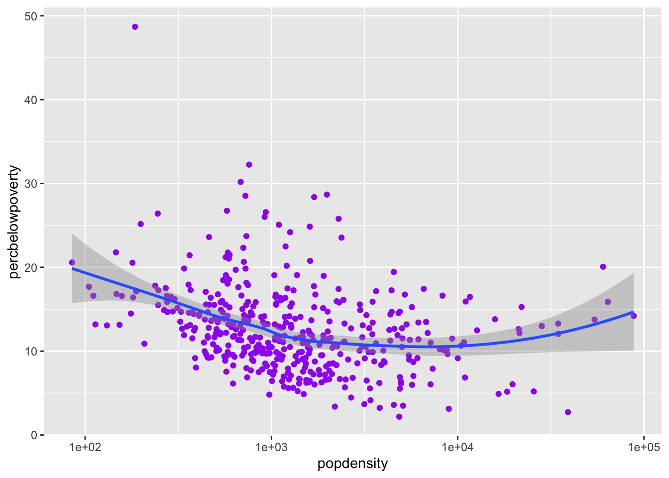
Histograms
ggplot(data = midwest,
       mapping = aes(x = percbelowpoverty)) +
  geom_histogram()
`stat_bin()` using `bins = 30`. Pick better value with `binwidth`.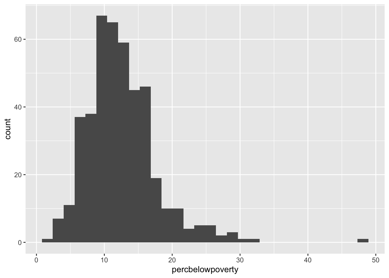
Data Wrangling (week 2-3)
Subsetting a data frame
Use the filter() function from the dplyr package to subset a data frame.
library(gov50data)

news |>
  filter(weekday == "Tue")
# A tibble: 509 × 10
callsign affiliation date weekday ideology national_politics
<chr> <chr> <date> <ord> <dbl> <dbl>
1 KAEF ABC 2017-06-13 Tue 0.0242 0.180
2 KBVU FOX 2017-06-13 Tue 0.00894 0.186
3 KBZK CBS 2017-06-13 Tue 0.129 0.306
4 KCVU FOX 2017-06-13 Tue 0.114 0.124
5 KECI NBC 2017-06-13 Tue 0.115 0.283
6 KHSL CBS 2017-06-13 Tue 0.0821 0.274
7 KNVN NBC 2017-06-13 Tue 0.120 0.261
8 KPAX CBS 2017-06-13 Tue 0.0984 0.208
9 KRCR ABC 2017-06-13 Tue 0.0187 0.206
10 KTMF ABC 2017-06-13 Tue 0.233 0.101
# ℹ 499 more rows
# ℹ 4 more variables: local_politics <dbl>, sinclair2017 <dbl>, post <dbl>,
# month <ord>You can filter based on multiple conditions to subset to the rows that meet all conditions:
news |>
  filter(weekday == "Tue",
         affiliation == "FOX")
# A tibble: 70 × 10
callsign affiliation date weekday ideology national_politics
<chr> <chr> <date> <ord> <dbl> <dbl>
1 KBVU FOX 2017-06-13 Tue 0.00894 0.186
2 KCVU FOX 2017-06-13 Tue 0.114 0.124
3 WEMT FOX 2017-06-13 Tue 0.235 0.149
4 WYDO FOX 2017-06-13 Tue 0.0949 0.182
5 WEMT FOX 2017-06-20 Tue 0.268 0.134
6 WYDO FOX 2017-06-20 Tue 0.0590 0.155
7 WEMT FOX 2017-06-27 Tue 0.0457 0.164
8 WYDO FOX 2017-06-27 Tue -0.0588 0.147
9 WEMT FOX 2017-07-04 Tue 0.0801 0.0986
10 WYDO FOX 2017-07-04 Tue 0.0555 0.0910
# ℹ 60 more rows
# ℹ 4 more variables: local_politics <dbl>, sinclair2017 <dbl>, post <dbl>,
# month <ord>You can use the | operator to match one of two conditions (“OR” rather than “AND”):
news |>
  filter(affiliation == "FOX" | affiliation == "ABC")
# A tibble: 1,033 × 10
callsign affiliation date weekday ideology national_politics
<chr> <chr> <date> <ord> <dbl> <dbl>
1 KTMF ABC 2017-06-07 Wed 0.0842 0.152
2 KTXS ABC 2017-06-07 Wed -0.000488 0.0925
3 KAEF ABC 2017-06-08 Thu 0.0426 0.213
4 KBVU FOX 2017-06-08 Thu -0.0860 0.169
5 KTMF ABC 2017-06-08 Thu 0.0433 0.179
6 KTXS ABC 2017-06-08 Thu 0.0627 0.158
7 WCTI ABC 2017-06-08 Thu 0.139 0.225
8 KAEF ABC 2017-06-09 Fri 0.0870 0.153
9 KTXS ABC 2017-06-09 Fri 0.0879 0.0790
10 WCTI ABC 2017-06-09 Fri 0.0667 0.182
# ℹ 1,023 more rows
# ℹ 4 more variables: local_politics <dbl>, sinclair2017 <dbl>, post <dbl>,
# month <ord>To test if a variable is one of several possible values, you can also use the %in% command:
news |>
  filter(weekday %in% c("Mon", "Fri"))
# A tibble: 1,021 × 10
callsign affiliation date weekday ideology national_politics
<chr> <chr> <date> <ord> <dbl> <dbl>
1 KAEF ABC 2017-06-09 Fri 0.0870 0.153
2 KECI NBC 2017-06-09 Fri 0.115 0.216
3 KPAX CBS 2017-06-09 Fri 0.0882 0.315
4 KRBC NBC 2017-06-09 Fri 0.0929 0.152
5 KTAB CBS 2017-06-09 Fri 0.0588 0.0711
6 KTXS ABC 2017-06-09 Fri 0.0879 0.0790
7 WCTI ABC 2017-06-09 Fri 0.0667 0.182
8 WITN NBC 2017-06-09 Fri -0.0683 0.146
9 WNCT CBS 2017-06-09 Fri -0.0181 0.126
10 WYDO FOX 2017-06-09 Fri -0.0330 0.0802
# ℹ 1,011 more rows
# ℹ 4 more variables: local_politics <dbl>, sinclair2017 <dbl>, post <dbl>,
# month <ord>If you want to subset to a set of specific row numbers, you can use the slice function:
## subset to the first 5 rows
news |>
  slice(1:5)
# A tibble: 5 × 10
callsign affiliation date weekday ideology national_politics
<chr> <chr> <date> <ord> <dbl> <dbl>
1 KECI NBC 2017-06-07 Wed 0.0655 0.225
2 KPAX CBS 2017-06-07 Wed 0.0853 0.283
3 KRBC NBC 2017-06-07 Wed 0.0183 0.130
4 KTAB CBS 2017-06-07 Wed 0.0850 0.0901
5 KTMF ABC 2017-06-07 Wed 0.0842 0.152
# ℹ 4 more variables: local_politics <dbl>, sinclair2017 <dbl>, post <dbl>,
# month <ord>Here the 1:5 syntax tells R to produce a vector that starts at 1 and ends at 5, incrementing by 1:
1:5[1] 1 2 3 4 5Filtering to the largest/smallest values of a variable
To subset to the rows that have the largest or smallest values of a given variable, use the slice_max and slice_max functions. For the largest values, use slice_max and use the n argument to specify how many rows you want:
news |>
  slice_max(ideology, n = 5)
# A tibble: 5 × 10
callsign affiliation date weekday ideology national_politics
<chr> <chr> <date> <ord> <dbl> <dbl>
1 KAEF ABC 2017-06-19 Mon 0.778 0.0823
2 WYDO FOX 2017-07-19 Wed 0.580 0.126
3 KRCR ABC 2017-10-03 Tue 0.566 0.123
4 KAEF ABC 2017-10-18 Wed 0.496 0.0892
5 KBVU FOX 2017-11-16 Thu 0.491 0.159
# ℹ 4 more variables: local_politics <dbl>, sinclair2017 <dbl>, post <dbl>,
# month <ord>To get lowest values, use slice_min:
news |>
  slice_min(ideology, n = 5)
# A tibble: 5 × 10
callsign affiliation date weekday ideology national_politics
<chr> <chr> <date> <ord> <dbl> <dbl>
1 KRBC NBC 2017-10-19 Thu -0.674 0.0731
2 WJHL CBS 2017-12-08 Fri -0.673 0.0364
3 KRBC NBC 2017-10-18 Wed -0.586 0.0470
4 KCVU FOX 2017-06-22 Thu -0.414 0.158
5 KRBC NBC 2017-12-11 Mon -0.365 0.0674
# ℹ 4 more variables: local_politics <dbl>, sinclair2017 <dbl>, post <dbl>,
# month <ord>Sorting rows by a variable
You can sort the rows of a data set using the arrange() function. By default, this will sort the rows from smallest to largest.
news |>
  arrange(ideology)
# A tibble: 2,560 × 10
callsign affiliation date weekday ideology national_politics
<chr> <chr> <date> <ord> <dbl> <dbl>
1 KRBC NBC 2017-10-19 Thu -0.674 0.0731
2 WJHL CBS 2017-12-08 Fri -0.673 0.0364
3 KRBC NBC 2017-10-18 Wed -0.586 0.0470
4 KCVU FOX 2017-06-22 Thu -0.414 0.158
5 KRBC NBC 2017-12-11 Mon -0.365 0.0674
6 KAEF ABC 2017-06-21 Wed -0.315 0.130
7 KTMF ABC 2017-12-01 Fri -0.303 0.179
8 KWYB ABC 2017-12-01 Fri -0.303 0.160
9 KTVM NBC 2017-09-01 Fri -0.302 0.0507
10 KNVN NBC 2017-12-08 Fri -0.299 0.121
# ℹ 2,550 more rows
# ℹ 4 more variables: local_politics <dbl>, sinclair2017 <dbl>, post <dbl>,
# month <ord>If you would like to sort the rows from largest to smallest (descending order), you can wrap the variable name with desc():
news |>
  arrange(desc(ideology))
# A tibble: 2,560 × 10
callsign affiliation date weekday ideology national_politics
<chr> <chr> <date> <ord> <dbl> <dbl>
1 KAEF ABC 2017-06-19 Mon 0.778 0.0823
2 WYDO FOX 2017-07-19 Wed 0.580 0.126
3 KRCR ABC 2017-10-03 Tue 0.566 0.123
4 KAEF ABC 2017-10-18 Wed 0.496 0.0892
5 KBVU FOX 2017-11-16 Thu 0.491 0.159
6 KTMF ABC 2017-11-06 Mon 0.455 0.138
7 KAEF ABC 2017-06-29 Thu 0.447 0.126
8 KPAX CBS 2017-11-23 Thu 0.437 0.125
9 KTAB CBS 2017-11-16 Thu 0.427 0.0631
10 KCVU FOX 2017-07-06 Thu 0.406 0.154
# ℹ 2,550 more rows
# ℹ 4 more variables: local_politics <dbl>, sinclair2017 <dbl>, post <dbl>,
# month <ord>Selecting/subsetting the columns
You can subset the data to only certain columns using the select() command:
news |>
  select(callsign, date, ideology)
# A tibble: 2,560 × 3
callsign date ideology
<chr> <date> <dbl>
1 KECI 2017-06-07 0.0655
2 KPAX 2017-06-07 0.0853
3 KRBC 2017-06-07 0.0183
4 KTAB 2017-06-07 0.0850
5 KTMF 2017-06-07 0.0842
6 KTXS 2017-06-07 -0.000488
7 KAEF 2017-06-08 0.0426
8 KBVU 2017-06-08 -0.0860
9 KECI 2017-06-08 0.0902
10 KPAX 2017-06-08 0.0668
# ℹ 2,550 more rowsIf you want to select a range of columns from, say, callsign to ideology, you can use the : operator:
news |>
  select(callsign:ideology)
# A tibble: 2,560 × 5
callsign affiliation date weekday ideology
<chr> <chr> <date> <ord> <dbl>
1 KECI NBC 2017-06-07 Wed 0.0655
2 KPAX CBS 2017-06-07 Wed 0.0853
3 KRBC NBC 2017-06-07 Wed 0.0183
4 KTAB CBS 2017-06-07 Wed 0.0850
5 KTMF ABC 2017-06-07 Wed 0.0842
6 KTXS ABC 2017-06-07 Wed -0.000488
7 KAEF ABC 2017-06-08 Thu 0.0426
8 KBVU FOX 2017-06-08 Thu -0.0860
9 KECI NBC 2017-06-08 Thu 0.0902
10 KPAX CBS 2017-06-08 Thu 0.0668
# ℹ 2,550 more rowsYou can remove a variable from the data set by using the minus sign - in front of it:
news |>
  select(-callsign)
# A tibble: 2,560 × 9
affiliation date weekday ideology national_politics local_politics
<chr> <date> <ord> <dbl> <dbl> <dbl>
1 NBC 2017-06-07 Wed 0.0655 0.225 0.148
2 CBS 2017-06-07 Wed 0.0853 0.283 0.123
3 NBC 2017-06-07 Wed 0.0183 0.130 0.189
4 CBS 2017-06-07 Wed 0.0850 0.0901 0.138
5 ABC 2017-06-07 Wed 0.0842 0.152 0.129
6 ABC 2017-06-07 Wed -0.000488 0.0925 0.0791
7 ABC 2017-06-08 Thu 0.0426 0.213 0.228
8 FOX 2017-06-08 Thu -0.0860 0.169 0.247
9 NBC 2017-06-08 Thu 0.0902 0.276 0.152
10 CBS 2017-06-08 Thu 0.0668 0.305 0.124
# ℹ 2,550 more rows
# ℹ 3 more variables: sinclair2017 <dbl>, post <dbl>, month <ord>You can also drop several variables using the c() function or the (a:b) syntax:
news |>
  select(-c(callsign, date, ideology))
# A tibble: 2,560 × 7
affiliation weekday national_politics local_politics sinclair2017 post month
<chr> <ord> <dbl> <dbl> <dbl> <dbl> <ord>
1 NBC Wed 0.225 0.148 1 0 Jun
2 CBS Wed 0.283 0.123 0 0 Jun
3 NBC Wed 0.130 0.189 0 0 Jun
4 CBS Wed 0.0901 0.138 0 0 Jun
5 ABC Wed 0.152 0.129 0 0 Jun
6 ABC Wed 0.0925 0.0791 1 0 Jun
7 ABC Thu 0.213 0.228 1 0 Jun
8 FOX Thu 0.169 0.247 1 0 Jun
9 NBC Thu 0.276 0.152 1 0 Jun
10 CBS Thu 0.305 0.124 0 0 Jun
# ℹ 2,550 more rowsnews |>
select(-(callsign:ideology))# A tibble: 2,560 × 5
national_politics local_politics sinclair2017 post month
<dbl> <dbl> <dbl> <dbl> <ord>
1 0.225 0.148 1 0 Jun
2 0.283 0.123 0 0 Jun
3 0.130 0.189 0 0 Jun
4 0.0901 0.138 0 0 Jun
5 0.152 0.129 0 0 Jun
6 0.0925 0.0791 1 0 Jun
7 0.213 0.228 1 0 Jun
8 0.169 0.247 1 0 Jun
9 0.276 0.152 1 0 Jun
10 0.305 0.124 0 0 Jun
# ℹ 2,550 more rowsYou can also select columns based on matching patterns in the names with functions like starts_with() or ends_with():
news |>
  select(ends_with("politics"))
# A tibble: 2,560 × 2
national_politics local_politics
<dbl> <dbl>
1 0.225 0.148
2 0.283 0.123
3 0.130 0.189
4 0.0901 0.138
5 0.152 0.129
6 0.0925 0.0791
7 0.213 0.228
8 0.169 0.247
9 0.276 0.152
10 0.305 0.124
# ℹ 2,550 more rowsThis code finds all variables with column names that end with the string “politics”. See the help page for select() for more information on different ways to select.
Renaming a variable
You can rename a variable useing the function rename(new_name = old_name):
news |>
  rename(call_sign = callsign)
# A tibble: 2,560 × 10
call_sign affiliation date weekday ideology national_politics
<chr> <chr> <date> <ord> <dbl> <dbl>
1 KECI NBC 2017-06-07 Wed 0.0655 0.225
2 KPAX CBS 2017-06-07 Wed 0.0853 0.283
3 KRBC NBC 2017-06-07 Wed 0.0183 0.130
4 KTAB CBS 2017-06-07 Wed 0.0850 0.0901
5 KTMF ABC 2017-06-07 Wed 0.0842 0.152
6 KTXS ABC 2017-06-07 Wed -0.000488 0.0925
7 KAEF ABC 2017-06-08 Thu 0.0426 0.213
8 KBVU FOX 2017-06-08 Thu -0.0860 0.169
9 KECI NBC 2017-06-08 Thu 0.0902 0.276
10 KPAX CBS 2017-06-08 Thu 0.0668 0.305
# ℹ 2,550 more rows
# ℹ 4 more variables: local_politics <dbl>, sinclair2017 <dbl>, post <dbl>,
# month <ord>Creating new variables
You can create new variables that are functions of old variables using the mutate() function:
news |> mutate(
  national_local_diff = national_politics - local_politics) |>
  select(callsign, date, national_politics, local_politics,
         national_local_diff)
# A tibble: 2,560 × 5
callsign date national_politics local_politics national_local_diff
<chr> <date> <dbl> <dbl> <dbl>
1 KECI 2017-06-07 0.225 0.148 0.0761
2 KPAX 2017-06-07 0.283 0.123 0.160
3 KRBC 2017-06-07 0.130 0.189 -0.0589
4 KTAB 2017-06-07 0.0901 0.138 -0.0476
5 KTMF 2017-06-07 0.152 0.129 0.0229
6 KTXS 2017-06-07 0.0925 0.0791 0.0134
7 KAEF 2017-06-08 0.213 0.228 -0.0151
8 KBVU 2017-06-08 0.169 0.247 -0.0781
9 KECI 2017-06-08 0.276 0.152 0.124
10 KPAX 2017-06-08 0.305 0.124 0.180
# ℹ 2,550 more rowsCreating new variables based on yes/no conditions
If you want to create a new variable that can take on two values based on a logical conditional, you should use the if_else() function inside of mutate(). For instance, if we want to create a more nicely labeled version of the sinclair2017 variable (which is 0/1), we could do:
news |>
  mutate(Ownership = if_else(sinclair2017 == 1,
                             "Acquired by Sinclair",
                             "Not Acquired")) |>
  select(callsign, affiliation, date, sinclair2017, Ownership)
# A tibble: 2,560 × 5
callsign affiliation date sinclair2017 Ownership
<chr> <chr> <date> <dbl> <chr>
1 KECI NBC 2017-06-07 1 Acquired by Sinclair
2 KPAX CBS 2017-06-07 0 Not Acquired
3 KRBC NBC 2017-06-07 0 Not Acquired
4 KTAB CBS 2017-06-07 0 Not Acquired
5 KTMF ABC 2017-06-07 0 Not Acquired
6 KTXS ABC 2017-06-07 1 Acquired by Sinclair
7 KAEF ABC 2017-06-08 1 Acquired by Sinclair
8 KBVU FOX 2017-06-08 1 Acquired by Sinclair
9 KECI NBC 2017-06-08 1 Acquired by Sinclair
10 KPAX CBS 2017-06-08 0 Not Acquired
# ℹ 2,550 more rowsSummarizing a variable
You can calculate summaries of variables in the data set using the summarize() function.
news |>
  summarize(
    avg_ideology = mean(ideology),
    sd_ideology = sd(ideology),
    median_ideology = median(ideology)
  )
# A tibble: 1 × 3
avg_ideology sd_ideology median_ideology
<dbl> <dbl> <dbl>
1 0.0907 0.0962 0.0929Summarizing variables by groups of rows
By default, summarize() calculates the summaries of variables for all rows in the data frame. You can also calculate these summaries within groups of rows defined by another variable in the data frame using the group_by() function before summarizing.
news |>
  group_by(month) |>
  summarize(
    avg_ideology = mean(ideology),
    sd_ideology = sd(ideology),
    median_ideology = median(ideology)
  )
# A tibble: 7 × 4
month avg_ideology sd_ideology median_ideology
<ord> <dbl> <dbl> <dbl>
1 Jun 0.0786 0.0979 0.0838
2 Jul 0.103 0.0888 0.0992
3 Aug 0.105 0.0811 0.106
4 Sep 0.0751 0.0902 0.0768
5 Oct 0.0862 0.110 0.0853
6 Nov 0.0972 0.0893 0.102
7 Dec 0.0774 0.125 0.0878Here, the summarize() function breaks apart the original data into smaller data frames for each month and applies the summary functions to those, then combines everything into one tibble.
Summarizing by multiple variables
You can group by multiple variables and summarize() will create groups based on every combination of each variable:
news |>
  group_by(sinclair2017, post) |>
  summarize(
    avg_ideology = mean(ideology)
  )
`summarise()` has grouped output by 'sinclair2017'. You can override using the
`.groups` argument.# A tibble: 4 × 3
# Groups: sinclair2017 [2]
sinclair2017 post avg_ideology
<dbl> <dbl> <dbl>
1 0 0 0.100
2 0 1 0.0768
3 1 0 0.0936
4 1 1 0.0938You’ll notice the message that summarize() sends after using to let us know that resulting tibble is grouped by sinclair2017. By default, summarize() drops the last group you provided in group_by (post in this case). This isn’t an error message, it’s just letting us know some helpful information. If you want to avoid this messaging displaying, you need to specify what grouping you want after using the .groups argument:
news |>
  group_by(sinclair2017, post) |>
  summarize(
    avg_ideology = mean(ideology),
    .groups = "drop_last"
  )
# A tibble: 4 × 3
# Groups: sinclair2017 [2]
sinclair2017 post avg_ideology
<dbl> <dbl> <dbl>
1 0 0 0.100
2 0 1 0.0768
3 1 0 0.0936
4 1 1 0.0938Summarizing across many variables
If you want to apply the same summary to multiple variables, you can use the across(vars, fun) function, where vars is a vector of variable names (specified like with select()) and fun is a summary function to apply to those variables.
news |>
  group_by(sinclair2017, post) |>
  summarize(
    across(c(ideology, national_politics), mean)
  )
`summarise()` has grouped output by 'sinclair2017'. You can override using the
`.groups` argument.# A tibble: 4 × 4
# Groups: sinclair2017 [2]
sinclair2017 post ideology national_politics
<dbl> <dbl> <dbl> <dbl>
1 0 0 0.100 0.134
2 0 1 0.0768 0.126
3 1 0 0.0936 0.137
4 1 1 0.0938 0.155As with select(), you can use the : operator to select a range of variables
news |>
  group_by(sinclair2017, post) |>
  summarize(
    across(ideology:local_politics, mean)
  )
`summarise()` has grouped output by 'sinclair2017'. You can override using the
`.groups` argument.# A tibble: 4 × 5
# Groups: sinclair2017 [2]
sinclair2017 post ideology national_politics local_politics
<dbl> <dbl> <dbl> <dbl> <dbl>
1 0 0 0.100 0.134 0.168
2 0 1 0.0768 0.126 0.167
3 1 0 0.0936 0.137 0.157
4 1 1 0.0938 0.155 0.139Table of counts of a categorical variable
There are two way to produce a table of counts of each category of a variable. The first is to use group_by and summarize along with the summary function n(), which returns the numbers of rows in each grouping (that is, each combination of the grouping variables):
news |>
  group_by(affiliation) |>
  summarize(n = n())
# A tibble: 4 × 2
affiliation n
<chr> <int>
1 ABC 687
2 CBS 758
3 FOX 346
4 NBC 769A simpler way to acheive the same outcome is to use the count() function, which implements these two steps:
news |>
  count(affiliation)
# A tibble: 4 × 2
affiliation n
<chr> <int>
1 ABC 687
2 CBS 758
3 FOX 346
4 NBC 769Producing nicely formatted tables with kable()
You can take any tibble in R and convert it into a more readable output by passing it to knitr::kable(). In our homework, generally, we will save the tibble as an object and then pass it to this function.
month_summary <- news |>
  group_by(month) |>
  summarize(
    avg_ideology = mean(ideology),
    sd_ideology = sd(ideology)
  )

knitr::kable(month_summary)| month | avg_ideology | sd_ideology |
|---|---|---|
| Jun | 0.0785518 | 0.0979339 |
| Jul | 0.1032917 | 0.0888328 |
| Aug | 0.1049908 | 0.0811141 |
| Sep | 0.0751067 | 0.0902003 |
| Oct | 0.0861639 | 0.1098108 |
| Nov | 0.0971796 | 0.0892845 |
| Dec | 0.0773873 | 0.1246451 |
You can add informative column names to the table using the col.names argument.
knitr::kable(
  month_summary,
  col.names = c("Month", "Average Ideology", "SD of Ideology")
)| Month | Average Ideology | SD of Ideology |
|---|---|---|
| Jun | 0.0785518 | 0.0979339 |
| Jul | 0.1032917 | 0.0888328 |
| Aug | 0.1049908 | 0.0811141 |
| Sep | 0.0751067 | 0.0902003 |
| Oct | 0.0861639 | 0.1098108 |
| Nov | 0.0971796 | 0.0892845 |
| Dec | 0.0773873 | 0.1246451 |
Finally, we can round the numbers in the table to be a bit nicer using the digits argument. This will tell kable() how many significant digiits to show.
knitr::kable(
  month_summary,
  col.names = c("Month", "Average Ideology", "SD of Ideology"),
  digits = 3
)| Month | Average Ideology | SD of Ideology |
|---|---|---|
| Jun | 0.079 | 0.098 |
| Jul | 0.103 | 0.089 |
| Aug | 0.105 | 0.081 |
| Sep | 0.075 | 0.090 |
| Oct | 0.086 | 0.110 |
| Nov | 0.097 | 0.089 |
| Dec | 0.077 | 0.125 |
Barplots of counts
You can visualize counts of a variable using a barplot:
news |>
  ggplot(mapping = aes(x = affiliation)) +
  geom_bar()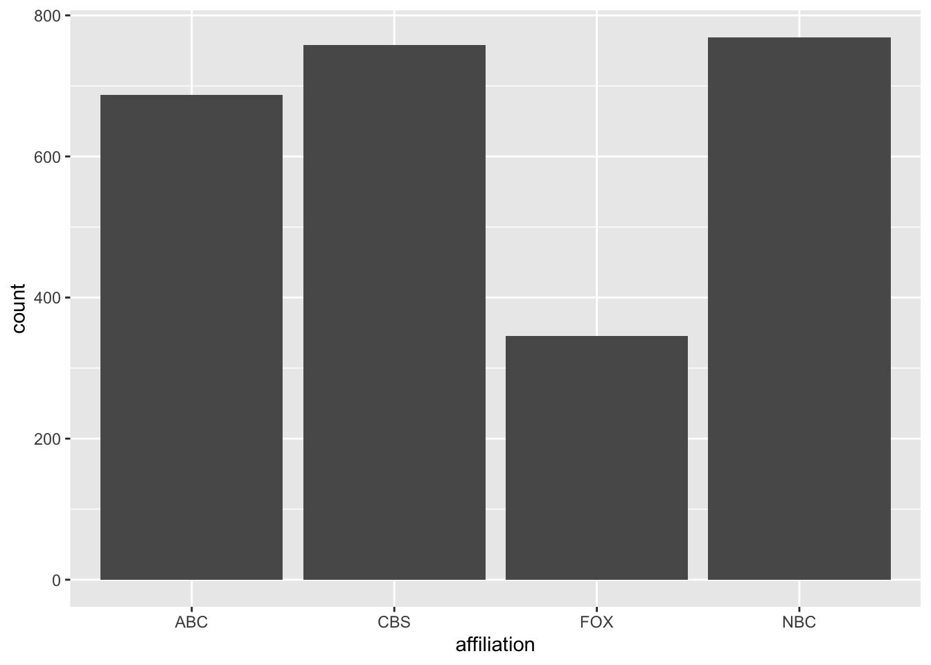
Barplots of other summaries
We can use barplots to visualize other grouped summaries like means, but we need to use the geom_col() geom instead and specify the variable you want to be the height of the bars .
news |>
  group_by(affiliation) |>
  summarize(
    avg_ideology = mean(ideology)
  ) |>
  ggplot(mapping = aes(x = affiliation, y = avg_ideology)) +
  geom_col()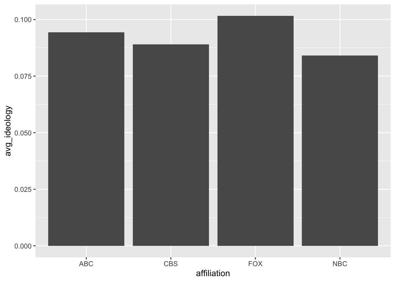
Reordering/sorting barplot axes
Often we want to sort the barplot axes to be in the order of the variable of interest so we can quickly compare them. We can use the fct_reorder(group_var, ordering_var) function to do this where the group_var is the grouping variable that is going on the axes and the ordering_var is the variable that we will sort the groups on.
news |>
  group_by(affiliation) |>
  summarize(
    avg_ideology = mean(ideology)
  ) |>
  ggplot(mapping = aes(x = fct_reorder(affiliation, avg_ideology),
                       y = avg_ideology)) +
  geom_col()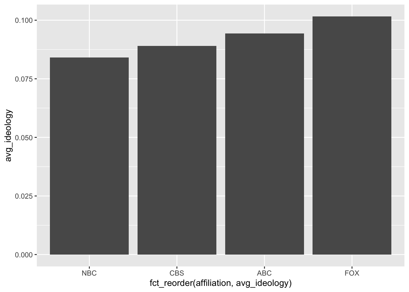
Coloring barplots by another variable
You can color the barplots by a another variable using the fill aesthetic:
news |>
  group_by(callsign, affiliation) |>
  summarize(
    avg_ideology = mean(ideology)
  ) |>
  slice_max(avg_ideology, n = 10) |>
  ggplot(mapping = aes(y = fct_reorder(callsign, avg_ideology),
                       x = avg_ideology)) +
  geom_col(mapping = aes(fill = affiliation))
`summarise()` has grouped output by 'callsign'. You can override using the
`.groups` argument.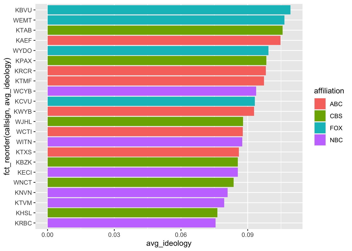
Creating logical vectors
You can create logical variables in your tibbles using mutate:
news |>
  mutate(
    right_leaning = ideology > 0,
    fall = month == "Sep" | month == "Oct" | month == "Nov",
    .keep = "used"
)
# A tibble: 2,560 × 4
ideology month right_leaning fall
<dbl> <ord> <lgl> <lgl>
1 0.0655 Jun TRUE FALSE
2 0.0853 Jun TRUE FALSE
3 0.0183 Jun TRUE FALSE
4 0.0850 Jun TRUE FALSE
5 0.0842 Jun TRUE FALSE
6 -0.000488 Jun FALSE FALSE
7 0.0426 Jun TRUE FALSE
8 -0.0860 Jun FALSE FALSE
9 0.0902 Jun TRUE FALSE
10 0.0668 Jun TRUE FALSE
# ℹ 2,550 more rowsThe .keep = "used" argument here tells mutate to only return the variables created and any variables used to create them. We’re using it here for display purposes.
You can filter based on these logical variables. In particular, if we want to subset to rows where both right_leaning and fall were TRUE we could do the following filter:
news |>
  mutate(
    right_leaning = ideology > 0,
    fall = month == "Sep" | month == "Oct" | month == "Nov",
    .keep = "used"
  ) |>
  filter(right_leaning & fall)
# A tibble: 1,050 × 4
ideology month right_leaning fall
<dbl> <ord> <lgl> <lgl>
1 0.121 Sep TRUE TRUE
2 0.0564 Sep TRUE TRUE
3 0.0564 Sep TRUE TRUE
4 0.324 Sep TRUE TRUE
5 0.0649 Sep TRUE TRUE
6 0.0613 Sep TRUE TRUE
7 0.187 Sep TRUE TRUE
8 0.0297 Sep TRUE TRUE
9 0.151 Sep TRUE TRUE
10 0.186 Sep TRUE TRUE
# ℹ 1,040 more rowsUsing ! to negate logicals
Any time you place the exclamation point in front of a logical, it will turn any TRUE into a FALSE and vice versa. For instance, if we wanted left leaning days in the fall, we could used
news |>
  mutate(
    right_leaning = ideology > 0,
    fall = month == "Sep" | month == "Oct" | month == "Nov",
    .keep = "used"
  ) |>
  filter(!right_leaning & fall)
# A tibble: 167 × 4
ideology month right_leaning fall
<dbl> <ord> <lgl> <lgl>
1 -0.0387 Sep FALSE TRUE
2 -0.302 Sep FALSE TRUE
3 -0.00694 Sep FALSE TRUE
4 -0.0140 Sep FALSE TRUE
5 -0.0294 Sep FALSE TRUE
6 -0.0113 Sep FALSE TRUE
7 -0.105 Sep FALSE TRUE
8 -0.0286 Sep FALSE TRUE
9 -0.0462 Sep FALSE TRUE
10 -0.0313 Sep FALSE TRUE
# ℹ 157 more rowsOr if we wanted to subset to any combination except right leaning and fall, we could negate the AND statement using parentheses:
news |>
  mutate(
    right_leaning = ideology > 0,
    fall = month == "Sep" | month == "Oct" | month == "Nov",
    .keep = "used"
  ) |>
  filter(!(right_leaning & fall))
# A tibble: 1,510 × 4
ideology month right_leaning fall
<dbl> <ord> <lgl> <lgl>
1 0.0655 Jun TRUE FALSE
2 0.0853 Jun TRUE FALSE
3 0.0183 Jun TRUE FALSE
4 0.0850 Jun TRUE FALSE
5 0.0842 Jun TRUE FALSE
6 -0.000488 Jun FALSE FALSE
7 0.0426 Jun TRUE FALSE
8 -0.0860 Jun FALSE FALSE
9 0.0902 Jun TRUE FALSE
10 0.0668 Jun TRUE FALSE
# ℹ 1,500 more rowsThis is often used in combination with %in% to acheive a “not in” logical:
news |>
  filter(!(affiliation %in% c("FOX", "ABC")))
# A tibble: 1,527 × 10
callsign affiliation date weekday ideology national_politics
<chr> <chr> <date> <ord> <dbl> <dbl>
1 KECI NBC 2017-06-07 Wed 0.0655 0.225
2 KPAX CBS 2017-06-07 Wed 0.0853 0.283
3 KRBC NBC 2017-06-07 Wed 0.0183 0.130
4 KTAB CBS 2017-06-07 Wed 0.0850 0.0901
5 KECI NBC 2017-06-08 Thu 0.0902 0.276
6 KPAX CBS 2017-06-08 Thu 0.0668 0.305
7 KRBC NBC 2017-06-08 Thu 0.108 0.156
8 KTAB CBS 2017-06-08 Thu -0.0178 0.0726
9 KECI NBC 2017-06-09 Fri 0.115 0.216
10 KPAX CBS 2017-06-09 Fri 0.0882 0.315
# ℹ 1,517 more rows
# ℹ 4 more variables: local_politics <dbl>, sinclair2017 <dbl>, post <dbl>,
# month <ord>Grouped summaries with any() and all()
Once you group a tibble, you can summarize logicals within groups using two commands. any() will return TRUE if a logical is TRUE for any row in a group and FALSE otherwise. all() will return TRUE when the logical inside it is TRUE for all rows in a group and FALSE otherwise.
news |>
  group_by(callsign) |>
  summarize(
    any_liberal = any(ideology < 0),
    all_local = all(national_politics < local_politics)
  )
# A tibble: 22 × 3
callsign any_liberal all_local
<chr> <lgl> <lgl>
1 KAEF TRUE FALSE
2 KBVU TRUE FALSE
3 KBZK TRUE FALSE
4 KCVU TRUE FALSE
5 KECI TRUE FALSE
6 KHSL TRUE FALSE
7 KNVN TRUE FALSE
8 KPAX TRUE FALSE
9 KRBC TRUE FALSE
10 KRCR TRUE FALSE
# ℹ 12 more rowsConverting logicals
When passed to sum() or mean(), TRUE is converted to 1 and FALSE is converted to 0. This means that sum() will return the number of TRUE values in a vector and mean() will return the proportion of TRUE values.
sum(c(TRUE, FALSE, TRUE, FALSE))[1] 2mean(c(TRUE, FALSE, TRUE, FALSE))[1] 0.5Grouped logical summaries with sums and means
After grouping, you can summarize using either the sum() or mean() function on a logical. In this case, the sum() will give you the number of time the statement is TRUE within a group, and mean() will give you the proportion of rows that are TRUE within a group.
news |>
  group_by(callsign) |>
  summarize(
    prop_liberal = mean(ideology < 0),
    num_local_bigger = sum(national_politics < local_politics)
  )
# A tibble: 22 × 3
callsign prop_liberal num_local_bigger
<chr> <dbl> <int>
1 KAEF 0.138 111
2 KBVU 0.143 31
3 KBZK 0.0526 11
4 KCVU 0.185 38
5 KECI 0.137 44
6 KHSL 0.132 127
7 KNVN 0.115 130
8 KPAX 0.0833 74
9 KRBC 0.196 103
10 KRCR 0.0992 99
# ℹ 12 more rowsCausality (Week 4)
For this week, we’ll use the data from the transphobia randomized experiment
trans# A tibble: 565 × 9
age female voted_gen_14 voted_gen_12 treat_ind racename democrat
<dbl> <dbl> <dbl> <dbl> <dbl> <chr> <dbl>
1 29 0 0 1 0 African American 1
2 59 1 1 0 1 African American 1
3 35 1 1 1 1 African American 1
4 63 1 1 1 1 African American 1
5 65 0 1 1 1 African American 0
6 51 1 1 1 0 Caucasian 0
7 26 1 1 1 0 African American 1
8 62 1 1 1 1 African American 1
9 37 0 1 1 0 Caucasian 0
10 51 1 1 1 0 Caucasian 0
# ℹ 555 more rows
# ℹ 2 more variables: nondiscrim_pre <dbl>, nondiscrim_post <dbl>Calculating a difference in means by filtering
You can calculate a difference in means by creating separate summaries of the treatment and control arms of an experiment or observational study and then taking the differences between them:
treat_mean <- trans |>
  filter(treat_ind == 1) |>
  summarize(nondiscrim_mean = mean(nondiscrim_post))
treat_mean
# A tibble: 1 × 1
nondiscrim_mean
<dbl>
1 0.687control_mean <- trans |>
filter(treat_ind == 0) |>
summarize(nondiscrim_mean = mean(nondiscrim_post))
control_mean# A tibble: 1 × 1
nondiscrim_mean
<dbl>
1 0.648diff_in_means <- treat_mean - control_mean
diff_in_means nondiscrim_mean
1 0.03896674Pivoting a tibble to make a cross-tab
When grouping by two variables, we sometimes would like the values of one variable to be in the rows and values of the other variable to be in the columns. But group_by() and summarize() by default puts each combination of values for the two variables into rows. We can use the pivot_wider function to move one of the variables (specified with the names_from argument) to the columns. The values_from argument tells R what variable should it use to fil in the data in the resulting table.
So if we wanted to get counts of race (rows) by treatment group (columns), we could start with getting the counts:
trans |>
  group_by(treat_ind, racename) |>
  summarize(n = n())
`summarise()` has grouped output by 'treat_ind'. You can override using the
`.groups` argument.# A tibble: 9 × 3
# Groups: treat_ind [2]
treat_ind racename n
<dbl> <chr> <int>
1 0 African American 58
2 0 Asian 2
3 0 Caucasian 77
4 0 Hispanic 150
5 1 African American 68
6 1 Asian 4
7 1 Caucasian 75
8 1 Hispanic 130
9 1 Native American 1Then we can pivot the treatment group to the columns:
trans |>
  group_by(treat_ind, racename) |>
  summarize(n = n()) |>
  pivot_wider(
    names_from = treat_ind,
    values_from = n
  )
`summarise()` has grouped output by 'treat_ind'. You can override using the
`.groups` argument.# A tibble: 5 × 3
racename `0` `1`
<chr> <int> <int>
1 African American 58 68
2 Asian 2 4
3 Caucasian 77 75
4 Hispanic 150 130
5 Native American NA 1Calculating difference in means by pivoting
Now that we know pivoting, we can use this to calculate difference in means instead of the filter approach. We first calculate the means by treatment group, pivot the rows to columns, and finally use mutate() to create the difference between the means.
trans |>
  group_by(treat_ind) |>
  summarize(nondiscrim_mean = mean(nondiscrim_post)) |>
  pivot_wider(
    names_from = treat_ind,
    values_from = nondiscrim_mean
  ) |>
  mutate(
    diff_in_means = `1` - `0`
  )
# A tibble: 1 × 3
`0` `1` diff_in_means
<dbl> <dbl> <dbl>
1 0.648 0.687 0.0390Creating new labels for variables to make nicer tables
Above we had to use the backticks to refer to the 1/0 variable names when calculating the differences in means. We can create slightly nicer output by relabeling the treat_ind variable using if_else:
trans |>
  mutate(
    treat_ind = if_else(treat_ind == 1, "Treated", "Control")
  ) |>
  group_by(treat_ind) |>
  summarize(nondiscrim_mean = mean(nondiscrim_post)) |>
  pivot_wider(
    names_from = treat_ind,
    values_from = nondiscrim_mean
  ) |>
  mutate(
    diff_in_means = Treated - Control
  )
# A tibble: 1 × 3
Control Treated diff_in_means
<dbl> <dbl> <dbl>
1 0.648 0.687 0.0390Calculating difference in means by two-level grouping variable
If we have a two-level grouping variable like democrat, we can create nice labels for that variable and just add it to the group_by call to get the difference in means within levels of this variable:
trans |>
  mutate(
    treat_ind = if_else(treat_ind == 1, "Treated", "Control"),
    party = if_else(democrat == 1, "Democrat", "Non-Democrat")
  ) |>
  group_by(treat_ind, party) |>
  summarize(nondiscrim_mean = mean(nondiscrim_post)) |>
  pivot_wider(
    names_from = treat_ind,
    values_from = nondiscrim_mean
  ) |>
  mutate(
    diff_in_means = Treated - Control
  )
`summarise()` has grouped output by 'treat_ind'. You can override using the
`.groups` argument.# A tibble: 2 × 4
party Control Treated diff_in_means
<chr> <dbl> <dbl> <dbl>
1 Democrat 0.704 0.754 0.0498
2 Non-Democrat 0.605 0.628 0.0234Creating grouping variables with more than 2 levels
You can use case_when() to create a variable that can take on more than 2 values based on conditions of a variable in the tibble:
trans |>
  mutate(
    age_group = case_when(
      age < 25 ~ "Under 25",
      age >=25 & age < 65 ~ "Bewteen 25 and 65",
      age >= 65 ~ "Older than 65"
    )
  ) |>
  select(age, age_group)
# A tibble: 565 × 2
age age_group
<dbl> <chr>
1 29 Bewteen 25 and 65
2 59 Bewteen 25 and 65
3 35 Bewteen 25 and 65
4 63 Bewteen 25 and 65
5 65 Older than 65
6 51 Bewteen 25 and 65
7 26 Bewteen 25 and 65
8 62 Bewteen 25 and 65
9 37 Bewteen 25 and 65
10 51 Bewteen 25 and 65
# ℹ 555 more rowsCalculating difference in mean by grouping variable with more than 2 levels
trans |>
  mutate(
    treat_ind = if_else(treat_ind == 1, "Treated", "Control"),
    age_group = case_when(
      age < 25 ~ "Under 25",
      age >=25 & age < 65 ~ "Bewteen 25 and 65",
      age >= 65 ~ "Older than 65"
    )
  ) |>
  group_by(treat_ind, age_group) |>
  summarize(nondiscrim_mean = mean(nondiscrim_post)) |>
  pivot_wider(
    names_from = treat_ind,
    values_from = nondiscrim_mean
  ) |>
  mutate(
    diff_in_means = Treated - Control
  )
`summarise()` has grouped output by 'treat_ind'. You can override using the
`.groups` argument.# A tibble: 3 × 4
age_group Control Treated diff_in_means
<chr> <dbl> <dbl> <dbl>
1 Bewteen 25 and 65 0.694 0.683 -0.0112
2 Older than 65 0.576 0.614 0.0378
3 Under 25 0.556 0.829 0.273 Calculating before and after difference in means
When we’re estimating causal effects using a before and after design, we can usually create a variable that is the change in the outcome over time for each row and then take the mean of that. For example, in the newspapers data we have the vote for Labour outcome before the treatment (1992) and after (1997):
newspapers |>
  filter(to_labour == 1) |>
  mutate(
    vote_change = vote_lab_97 - vote_lab_92
  ) |>
  summarize(avg_change = mean(vote_change))
# A tibble: 1 × 1
avg_change
<dbl>
1 0.190Calculating difference-in-differences estimator
When you want to use the difference in differences estimator, you simply need to take the difference between the average changes over time in the treatment group (to_labour == 1) and the control group (to_labour == 0). We can do this by adding a group_by step:
newspapers |>
  mutate(
    vote_change = vote_lab_97 - vote_lab_92,
    to_labour = if_else(to_labour == 1, "switched", "unswitched")
  ) |>
  group_by(to_labour) |>
  summarize(avg_change = mean(vote_change)) |>
  pivot_wider(
    names_from = to_labour,
    values_from = avg_change
  ) |>
  mutate(DID = switched - unswitched)
# A tibble: 1 × 3
switched unswitched DID
<dbl> <dbl> <dbl>
1 0.190 0.110 0.0796Summarizing data (Week 5)
Calculating the mean, median, and standard deviation
Many of the summary functions have intuitive names:
gapminder |>
  summarize(
    gdp_mean = mean(gdpPercap),
    gdp_median = median(gdpPercap),
    gdp_sd = sd(gdpPercap)
  )
# A tibble: 1 × 3
gdp_mean gdp_median gdp_sd
<dbl> <dbl> <dbl>
1 7215. 3532. 9857.You can also use these functions outside of a summarize() call by accessing variables with the $ operator:
mean(gapminder$gdpPercap)[1] 7215.327Adding a vertical line to a plot
You can layer on vertical lines to a ggplot using the geom_vline() function. For horizontal lines, use geom_hline().
ggplot(gapminder, aes(x = lifeExp)) +
  geom_histogram(binwidth = 1) +
  geom_vline(aes(xintercept = mean(lifeExp)), color = "indianred") +
  geom_vline(aes(xintercept = median(lifeExp)), color = "dodgerblue")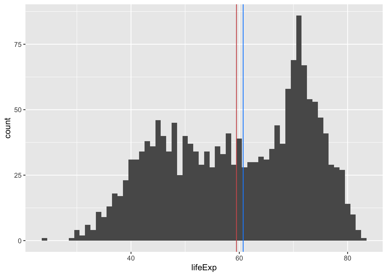
Dropping missing rows with missing data
To drop any row of a data frame with missing values in any variable, you can use the drop_na() function. Here we use the nrow() function to show how many rows each tibble has.
cces_2020 |>
  nrow()
[1] 51551cces_2020 |>
drop_na() |>
nrow()[1] 45651By default drop_na() drops rows that have any missingness. If you want to drop rows based on being missing only for a particular variable, just pass the variable name to the function:
cces_2020 |>
  drop_na(turnout_self) |>
  nrow()
[1] 48462Removing missing values in summary functions
Most summary functions have an argument na.rm (for “NA remove”) that is FALSE by default, meaning it tries to calculate summaries with missing values included:
cces_2020 |>
  summarize(avg_turnout = mean(turnout_self))
# A tibble: 1 × 1
avg_turnout
<dbl>
1 NATo remove missing values and calculate the summary based on the observed values for that variable, set na.rm = TRUE:
cces_2020 |>
  summarize(avg_turnout = mean(turnout_self, na.rm = TRUE))
# A tibble: 1 × 1
avg_turnout
<dbl>
1 0.942Detecting missing values
You cannot use x == NA for detecting missing values in R because it treats missing values quite literally and just returns NA for all values:
c(5, 6, NA, 0) == NA[1] NA NA NA NAInstead you can use is.na():
is.na(c(5, 6, NA, 0))[1] FALSE FALSE TRUE FALSEYou can negate this to test for non-missing values:
!is.na(c(5, 6, NA, 0))[1] TRUE TRUE FALSE TRUEUsing is.na to summarize missingness
Applying mean() to is.na() output will tell us the proportion of values in a vector that are missing. We can combine this with group_by and summarize to see what share of each party ID response are missing turnout:
cces_2020 |>
  group_by(pid3) |>
  summarize(
    missing_turnout = mean(is.na(turnout_self))
  )
# A tibble: 5 × 2
pid3 missing_turnout
<fct> <dbl>
1 Democrat 0.0280
2 Republican 0.0403
3 Independent 0.0718
4 Other 0.0709
5 Not sure 0.431 Proportion table for one variable
To get a proportion table for a single categorical variable, start with the approach to creating a table of counts of each category. Then just add a mutate() step to get the proportion:
cces_2020 |>
  group_by(pres_vote) |>
  summarize(n = n()) |>
  mutate(
    prop = n / sum(n)
  )
# A tibble: 7 × 3
pres_vote n prop
<fct> <int> <dbl>
1 Joe Biden (Democrat) 26188 0.508
2 Donald J. Trump (Republican) 17702 0.343
3 Other 1458 0.0283
4 I did not vote in this race 100 0.00194
5 I did not vote 13 0.000252
6 Not sure 190 0.00369
7 <NA> 5900 0.114 Proportion table with two variables
With two variables, we take the same approach as for one variable, but we need to be careful about the grouping:
cces_2020 |>
  filter(pres_vote %in% c("Joe Biden (Democrat)",
                          "Donald J. Trump (Republican)")) |>
  group_by(pid3, pres_vote) |>
  summarize(n = n()) |>
  mutate(prop = n / sum(n))
`summarise()` has grouped output by 'pid3'. You can override using the
`.groups` argument.# A tibble: 10 × 4
# Groups: pid3 [5]
pid3 pres_vote n prop
<fct> <fct> <int> <dbl>
1 Democrat Joe Biden (Democrat) 17649 0.968
2 Democrat Donald J. Trump (Republican) 581 0.0319
3 Republican Joe Biden (Democrat) 856 0.0712
4 Republican Donald J. Trump (Republican) 11164 0.929
5 Independent Joe Biden (Democrat) 6601 0.571
6 Independent Donald J. Trump (Republican) 4951 0.429
7 Other Joe Biden (Democrat) 735 0.487
8 Other Donald J. Trump (Republican) 774 0.513
9 Not sure Joe Biden (Democrat) 347 0.599
10 Not sure Donald J. Trump (Republican) 232 0.401 After summarizing, the tibble drops the last grouping variable and groups the resulting tibble by the remaining variable(s). In this case, pres_vote is dropped and the tibble is now grouped by pid3. This means that when we call mutate(), the calculations will be done within levels of pid3. So the first row here is telling us the the share of Democrats that voted for Biden is 0.968.
If we want to have the proportion be as a share of the pres_vote instead, we can reorder the grouping variables:
cces_2020 |>
  filter(pres_vote %in% c("Joe Biden (Democrat)",
                          "Donald J. Trump (Republican)")) |>
  group_by(pres_vote, pid3) |>
  summarize(n = n()) |>
  mutate(prop = n / sum(n))
`summarise()` has grouped output by 'pres_vote'. You can override using the
`.groups` argument.# A tibble: 10 × 4
# Groups: pres_vote [2]
pres_vote pid3 n prop
<fct> <fct> <int> <dbl>
1 Joe Biden (Democrat) Democrat 17649 0.674
2 Joe Biden (Democrat) Republican 856 0.0327
3 Joe Biden (Democrat) Independent 6601 0.252
4 Joe Biden (Democrat) Other 735 0.0281
5 Joe Biden (Democrat) Not sure 347 0.0133
6 Donald J. Trump (Republican) Democrat 581 0.0328
7 Donald J. Trump (Republican) Republican 11164 0.631
8 Donald J. Trump (Republican) Independent 4951 0.280
9 Donald J. Trump (Republican) Other 774 0.0437
10 Donald J. Trump (Republican) Not sure 232 0.0131Finally, if we want the proportions to be out of all rows of the data, we can tell summarize() to drop the grouping:
cces_2020 |>
  filter(pres_vote %in% c("Joe Biden (Democrat)",
                          "Donald J. Trump (Republican)")) |>
  group_by(pid3, pres_vote) |>
  summarize(n = n(), .groups = "drop") |>
  mutate(prop = n / sum(n))
# A tibble: 10 × 4
pid3 pres_vote n prop
<fct> <fct> <int> <dbl>
1 Democrat Joe Biden (Democrat) 17649 0.402
2 Democrat Donald J. Trump (Republican) 581 0.0132
3 Republican Joe Biden (Democrat) 856 0.0195
4 Republican Donald J. Trump (Republican) 11164 0.254
5 Independent Joe Biden (Democrat) 6601 0.150
6 Independent Donald J. Trump (Republican) 4951 0.113
7 Other Joe Biden (Democrat) 735 0.0167
8 Other Donald J. Trump (Republican) 774 0.0176
9 Not sure Joe Biden (Democrat) 347 0.00791
10 Not sure Donald J. Trump (Republican) 232 0.00529Create cross-tab proportion tables
We can pivot our proportion tables to create cross-tabs, but if we leave in the count variable, we get output that we don’t expect:
cces_2020 |>
  filter(pres_vote %in% c("Joe Biden (Democrat)",
                          "Donald J. Trump (Republican)")) |>
  group_by(pid3, pres_vote) |>
  summarize(n = n()) |>
  mutate(prop = n / sum(n)) |>
  pivot_wider(
    names_from = pres_vote,
    values_from = prop
  )
`summarise()` has grouped output by 'pid3'. You can override using the
`.groups` argument.# A tibble: 10 × 4
# Groups: pid3 [5]
pid3 n `Joe Biden (Democrat)` `Donald J. Trump (Republican)`
<fct> <int> <dbl> <dbl>
1 Democrat 17649 0.968 NA
2 Democrat 581 NA 0.0319
3 Republican 856 0.0712 NA
4 Republican 11164 NA 0.929
5 Independent 6601 0.571 NA
6 Independent 4951 NA 0.429
7 Other 735 0.487 NA
8 Other 774 NA 0.513
9 Not sure 347 0.599 NA
10 Not sure 232 NA 0.401 To combat this, we can either drop the count variable:
cces_2020 |>
  filter(pres_vote %in% c("Joe Biden (Democrat)",
                          "Donald J. Trump (Republican)")) |>
  group_by(pid3, pres_vote) |>
  summarize(n = n()) |>
  mutate(prop = n / sum(n)) |>
  select(-n) |>
  pivot_wider(
    names_from = pres_vote,
    values_from = prop
  )
`summarise()` has grouped output by 'pid3'. You can override using the
`.groups` argument.# A tibble: 5 × 3
# Groups: pid3 [5]
pid3 `Joe Biden (Democrat)` `Donald J. Trump (Republican)`
<fct> <dbl> <dbl>
1 Democrat 0.968 0.0319
2 Republican 0.0712 0.929
3 Independent 0.571 0.429
4 Other 0.487 0.513
5 Not sure 0.599 0.401 Or we can also be specific about what variables we want on the rows. We can use the id_cols argument to specify just the variables that will go on the rows:
cces_2020 |>
  filter(pres_vote %in% c("Joe Biden (Democrat)",
                          "Donald J. Trump (Republican)")) |>
  group_by(pid3, pres_vote) |>
  summarize(n = n()) |>
  mutate(prop = n / sum(n)) |>
  pivot_wider(
    id_cols = pid3,
    names_from = pres_vote,
    values_from = prop
  )
`summarise()` has grouped output by 'pid3'. You can override using the
`.groups` argument.# A tibble: 5 × 3
# Groups: pid3 [5]
pid3 `Joe Biden (Democrat)` `Donald J. Trump (Republican)`
<fct> <dbl> <dbl>
1 Democrat 0.968 0.0319
2 Republican 0.0712 0.929
3 Independent 0.571 0.429
4 Other 0.487 0.513
5 Not sure 0.599 0.401 Visualizing a proportion table
We can visualize our proportion table using by mapping the grouping variable to the x axis and the non-grouped variable to the fill aesthetic. We also need to use the position = "dodge" argument to the geom_col() function so that the two columns in each group don’t overlap.
cces_2020 |>
  filter(pres_vote %in% c("Joe Biden (Democrat)",
                          "Donald J. Trump (Republican)")) |>
  mutate(pres_vote = if_else(pres_vote == "Joe Biden (Democrat)",
                             "Biden", "Trump")) |>
  group_by(pid3, pres_vote) |>
  summarize(n = n()) |>
  mutate(prop = n / sum(n)) |>

ggplot(aes(x = pid3, y = prop, fill = pres_vote)) +
  geom_col(position = "dodge") +
  scale_fill_manual(values = c(Biden = "steelblue1", Trump = "indianred1"))
`summarise()` has grouped output by 'pid3'. You can override using the
`.groups` argument.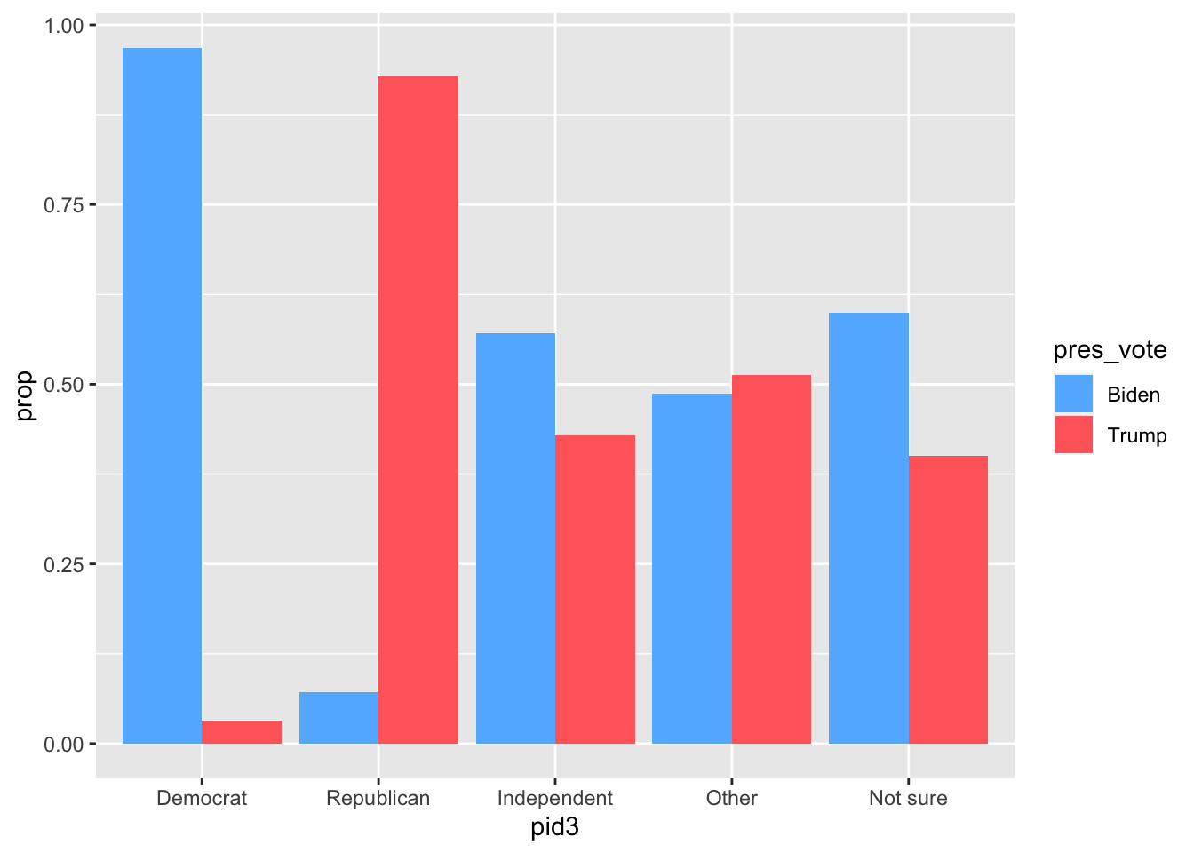
Bivariate Relationships and Joins (Week 6)
Calculating a correlation
You can calcuate a correlation between two variables using the cor function:
cor(news$national_politics, news$local_politics)[1] -0.05994132You can also use the pipe and summarize:
news |>
  summarize(cor(national_politics, local_politics))
# A tibble: 1 × 1
`cor(national_politics, local_politics)`
<dbl>
1 -0.0599When there are missing values in one of the variables, the correlation will be NA:
cor(covid_votes$one_dose_5plus_pct, covid_votes$dem_pct_2020)[1] NAIn that case, you can use the argument use = "pairwise" to remove the observations with missing values:
cor(covid_votes$one_dose_5plus_pct, covid_votes$dem_pct_2020,
    use = "pairwise")
[1] 0.6664387Writing a function
You can create a function with the function() function (oof). The arguments in the function() call will become the arguments of your function. For example, if we want to create a z-score function that takes in a vector and coverts it to a z-score, we can create a function for this:
z_score <- function(x) {
  (x - mean(x, na.rm = TRUE)) / sd(x, na.rm = TRUE)
}
Here, x is the argument that takes in the vector and it is used inside the function body to perform the task. Let’s call the function:
z_score(x = c(1, 2, 3, 4, 5))[1] -1.2649111 -0.6324555 0.0000000 0.6324555 1.2649111What happens here is that R runs the code inside the function definition, replacing x with the vector we pass to x, which in this case is c(1, 2, 3, 4, 5).
Pivoting longer
We sometimes have data that has data in the column names that we would actually like to be in the data frame itself. When this happens, we need the opposite of pivot_wider which is called pivot_longer. For example, the mortality data has the years in the column names, but we want the rows to be country-years:
mortality# A tibble: 217 × 52
country country_code indicator `1972` `1973` `1974` `1975` `1976` `1977`
<chr> <chr> <chr> <dbl> <dbl> <dbl> <dbl> <dbl> <dbl>
1 Aruba ABW Mortalit… NA NA NA NA NA NA
2 Afghanistan AFG Mortalit… 291 285. 280. 274. 268 262.
3 Angola AGO Mortalit… NA NA NA NA NA NA
4 Albania ALB Mortalit… NA NA NA NA NA NA
5 Andorra AND Mortalit… NA NA NA NA NA NA
6 United Arab… ARE Mortalit… 80.1 72.6 65.7 59.4 53.6 48.3
7 Argentina ARG Mortalit… 69.7 68.2 66.1 63.3 59.8 55.7
8 Armenia ARM Mortalit… NA NA NA NA 87.1 83.6
9 American Sa… ASM Mortalit… NA NA NA NA NA NA
10 Antigua and… ATG Mortalit… 26.9 25.1 23.5 22.1 20.8 19.5
# ℹ 207 more rows
# ℹ 43 more variables: `1978` <dbl>, `1979` <dbl>, `1980` <dbl>, `1981` <dbl>,
# `1982` <dbl>, `1983` <dbl>, `1984` <dbl>, `1985` <dbl>, `1986` <dbl>,
# `1987` <dbl>, `1988` <dbl>, `1989` <dbl>, `1990` <dbl>, `1991` <dbl>,
# `1992` <dbl>, `1993` <dbl>, `1994` <dbl>, `1995` <dbl>, `1996` <dbl>,
# `1997` <dbl>, `1998` <dbl>, `1999` <dbl>, `2000` <dbl>, `2001` <dbl>,
# `2002` <dbl>, `2003` <dbl>, `2004` <dbl>, `2005` <dbl>, `2006` <dbl>, …We can use pivot_longer to move this information. To do so, we need to pass the variables we want to pivot to the cols argument, the name of the new variable to hold the colum names into names_to, and the name of the column to hold the pivoted data in values_to.
mortality_long <- mortality |>
  select(-indicator) |>
  pivot_longer(
    cols = `1972`:`2020`,
    names_to = "year",
    values_to = "child_mortality"
  ) |>
  mutate(year = as.integer(year))
mortality_long
# A tibble: 10,633 × 4
country country_code year child_mortality
<chr> <chr> <int> <dbl>
1 Aruba ABW 1972 NA
2 Aruba ABW 1973 NA
3 Aruba ABW 1974 NA
4 Aruba ABW 1975 NA
5 Aruba ABW 1976 NA
6 Aruba ABW 1977 NA
7 Aruba ABW 1978 NA
8 Aruba ABW 1979 NA
9 Aruba ABW 1980 NA
10 Aruba ABW 1981 NA
# ℹ 10,623 more rowsHere we mutate the years to be integers because they are characters when initially pivoted.
Pivoting longer with a column name prefix
Sometimes the column names have a prefix in front of the data that we want, like in the spotify data where the week columns are all weekX where X is the week number. We’d like to extract X:
spotify# A tibble: 490 × 54
`Track Name` Artist week1 week2 week3 week4 week5 week6 week7 week8 week9
<chr> <chr> <dbl> <dbl> <dbl> <dbl> <dbl> <dbl> <dbl> <dbl> <dbl>
1 The Box Roddy… 1 1 1 1 1 1 1 1 1
2 ROXANNE Arizo… 2 4 5 4 4 4 6 7 9
3 Yummy Justi… 3 6 17 17 17 24 15 32 NA
4 Circles Post … 4 7 9 10 7 10 11 10 17
5 BOP DaBaby 5 5 7 5 11 12 18 18 32
6 Falling Trevo… 6 8 10 7 6 8 10 11 18
7 Dance Monkey Tones… 7 13 13 12 12 13 17 13 21
8 Bandit (with Yo… Juice… 8 11 14 14 15 20 27 26 42
9 Futsal Shuffle … Lil U… 9 9 19 21 24 32 40 49 NA
10 everything i wa… Billi… 10 17 28 9 8 11 14 17 29
# ℹ 480 more rows
# ℹ 43 more variables: week10 <dbl>, week11 <dbl>, week12 <dbl>, week13 <dbl>,
# week14 <dbl>, week15 <dbl>, week16 <dbl>, week17 <dbl>, week18 <dbl>,
# week19 <dbl>, week20 <dbl>, week21 <dbl>, week22 <dbl>, week23 <dbl>,
# week24 <dbl>, week25 <dbl>, week26 <dbl>, week27 <dbl>, week28 <dbl>,
# week29 <dbl>, week30 <dbl>, week31 <dbl>, week32 <dbl>, week33 <dbl>,
# week34 <dbl>, week35 <dbl>, week36 <dbl>, week37 <dbl>, week38 <dbl>, …We can use the names_prefix arugment to do this:
spotify |>
  pivot_longer(
    cols = c(-`Track Name`, -Artist),
    names_to = "week_of_year",
    values_to = "rank",
    names_prefix = "week"
  ) |>
  mutate(
    week_of_year = as.integer(week_of_year)
  )
# A tibble: 25,480 × 4
`Track Name` Artist week_of_year rank
<chr> <chr> <int> <dbl>
1 The Box Roddy Ricch 1 1
2 The Box Roddy Ricch 2 1
3 The Box Roddy Ricch 3 1
4 The Box Roddy Ricch 4 1
5 The Box Roddy Ricch 5 1
6 The Box Roddy Ricch 6 1
7 The Box Roddy Ricch 7 1
8 The Box Roddy Ricch 8 1
9 The Box Roddy Ricch 9 1
10 The Box Roddy Ricch 10 1
# ℹ 25,470 more rowsMerging one data frame into another (joins)
We can take the variables from one data frame and put them into another data frame using the various join functions. If we think of the primary data frame as A and the donor data frame as B, then if we want to keep the rows of A the same and just import the columns of B, then we can use the left_join
gapminder |>
  left_join(mortality_long)
Joining with `by = join_by(country, year)`# A tibble: 1,704 × 8
country continent year lifeExp pop gdpPercap country_code child_mortality
<chr> <fct> <int> <dbl> <int> <dbl> <chr> <dbl>
1 Afghan… Asia 1952 28.8 8.43e6 779. <NA> NA
2 Afghan… Asia 1957 30.3 9.24e6 821. <NA> NA
3 Afghan… Asia 1962 32.0 1.03e7 853. <NA> NA
4 Afghan… Asia 1967 34.0 1.15e7 836. <NA> NA
5 Afghan… Asia 1972 36.1 1.31e7 740. AFG 291
6 Afghan… Asia 1977 38.4 1.49e7 786. AFG 262.
7 Afghan… Asia 1982 39.9 1.29e7 978. AFG 231.
8 Afghan… Asia 1987 40.8 1.39e7 852. AFG 198.
9 Afghan… Asia 1992 41.7 1.63e7 649. AFG 166.
10 Afghan… Asia 1997 41.8 2.22e7 635. AFG 142.
# ℹ 1,694 more rowsBy default this keeps all rows of A and any rows in A that do not appear in B give missing values for the newly imported columns of B. If we want only the rows that are in both A and B, we can use inner_join
gapminder |>
  inner_join(mortality_long)
Joining with `by = join_by(country, year)`# A tibble: 1,048 × 8
country continent year lifeExp pop gdpPercap country_code child_mortality
<chr> <fct> <int> <dbl> <int> <dbl> <chr> <dbl>
1 Afghan… Asia 1972 36.1 1.31e7 740. AFG 291
2 Afghan… Asia 1977 38.4 1.49e7 786. AFG 262.
3 Afghan… Asia 1982 39.9 1.29e7 978. AFG 231.
4 Afghan… Asia 1987 40.8 1.39e7 852. AFG 198.
5 Afghan… Asia 1992 41.7 1.63e7 649. AFG 166.
6 Afghan… Asia 1997 41.8 2.22e7 635. AFG 142.
7 Afghan… Asia 2002 42.1 2.53e7 727. AFG 121.
8 Afghan… Asia 2007 43.8 3.19e7 975. AFG 99.9
9 Albania Europe 1972 67.7 2.26e6 3313. ALB NA
10 Albania Europe 1977 68.9 2.51e6 3533. ALB NA
# ℹ 1,038 more rowsSpecifying the key variables for a join
By default, the join functions will merge data frames A and B based on the columns that have the same name in both data frames. This sometimes isn’t what we want. For example, using the nycflights13 package, we might want to merge the flights and planes data frames. Both of these data sets have a year variable but they mean different things in the two data frames (the year of the flights vs the year the plane was manufactured):
library(nycflights13)
flights
# A tibble: 336,776 × 19
year month day dep_time sched_dep_time dep_delay arr_time sched_arr_time
<int> <int> <int> <int> <int> <dbl> <int> <int>
1 2013 1 1 517 515 2 830 819
2 2013 1 1 533 529 4 850 830
3 2013 1 1 542 540 2 923 850
4 2013 1 1 544 545 -1 1004 1022
5 2013 1 1 554 600 -6 812 837
6 2013 1 1 554 558 -4 740 728
7 2013 1 1 555 600 -5 913 854
8 2013 1 1 557 600 -3 709 723
9 2013 1 1 557 600 -3 838 846
10 2013 1 1 558 600 -2 753 745
# ℹ 336,766 more rows
# ℹ 11 more variables: arr_delay <dbl>, carrier <chr>, flight <int>,
# tailnum <chr>, origin <chr>, dest <chr>, air_time <dbl>, distance <dbl>,
# hour <dbl>, minute <dbl>, time_hour <dttm>planes# A tibble: 3,322 × 9
tailnum year type manufacturer model engines seats speed engine
<chr> <int> <chr> <chr> <chr> <int> <int> <int> <chr>
1 N10156 2004 Fixed wing multi… EMBRAER EMB-… 2 55 NA Turbo…
2 N102UW 1998 Fixed wing multi… AIRBUS INDU… A320… 2 182 NA Turbo…
3 N103US 1999 Fixed wing multi… AIRBUS INDU… A320… 2 182 NA Turbo…
4 N104UW 1999 Fixed wing multi… AIRBUS INDU… A320… 2 182 NA Turbo…
5 N10575 2002 Fixed wing multi… EMBRAER EMB-… 2 55 NA Turbo…
6 N105UW 1999 Fixed wing multi… AIRBUS INDU… A320… 2 182 NA Turbo…
7 N107US 1999 Fixed wing multi… AIRBUS INDU… A320… 2 182 NA Turbo…
8 N108UW 1999 Fixed wing multi… AIRBUS INDU… A320… 2 182 NA Turbo…
9 N109UW 1999 Fixed wing multi… AIRBUS INDU… A320… 2 182 NA Turbo…
10 N110UW 1999 Fixed wing multi… AIRBUS INDU… A320… 2 182 NA Turbo…
# ℹ 3,312 more rowsIn this case, we want to specify what variable we want to do the merge with. Here, we want to merge based on tailnum:
flights |>
  left_join(planes, by = "tailnum") |>
  select(year.x, tailnum, origin, dest, carrier, type, engine)
# A tibble: 336,776 × 7
year.x tailnum origin dest carrier type engine
<int> <chr> <chr> <chr> <chr> <chr> <chr>
1 2013 N14228 EWR IAH UA Fixed wing multi engine Turbo-fan
2 2013 N24211 LGA IAH UA Fixed wing multi engine Turbo-fan
3 2013 N619AA JFK MIA AA Fixed wing multi engine Turbo-fan
4 2013 N804JB JFK BQN B6 Fixed wing multi engine Turbo-fan
5 2013 N668DN LGA ATL DL Fixed wing multi engine Turbo-fan
6 2013 N39463 EWR ORD UA Fixed wing multi engine Turbo-fan
7 2013 N516JB EWR FLL B6 Fixed wing multi engine Turbo-fan
8 2013 N829AS LGA IAD EV Fixed wing multi engine Turbo-fan
9 2013 N593JB JFK MCO B6 Fixed wing multi engine Turbo-fan
10 2013 N3ALAA LGA ORD AA <NA> <NA>
# ℹ 336,766 more rowsBecause both data sets had a year variable, the join function renames them to year.x in the first data frame and year.y for the second. We could rename them before merging to solve this problem.
Regression (Week 8)
Add binned means to a scatterplot
You can add binned means of the y-axis variable in a scatterplot using the stat_summary_bin(fun = "mean") function with your ggplot call:
ggplot(health, aes(x = steps_lag, y = weight)) +
  geom_point(color = "steelblue1", alpha = 0.25) +
  labs(
    x = "Steps on day prior (in 1000s)",
    y = "Weight",
    title = "Weight and Steps"
  ) +
  stat_summary_bin(fun = "mean", color = "indianred1", size = 3,
                   geom = "point", binwidth = 1)
Warning: Removed 1 rows containing non-finite values (`stat_summary_bin()`).Warning: Removed 1 rows containing missing values (`geom_point()`).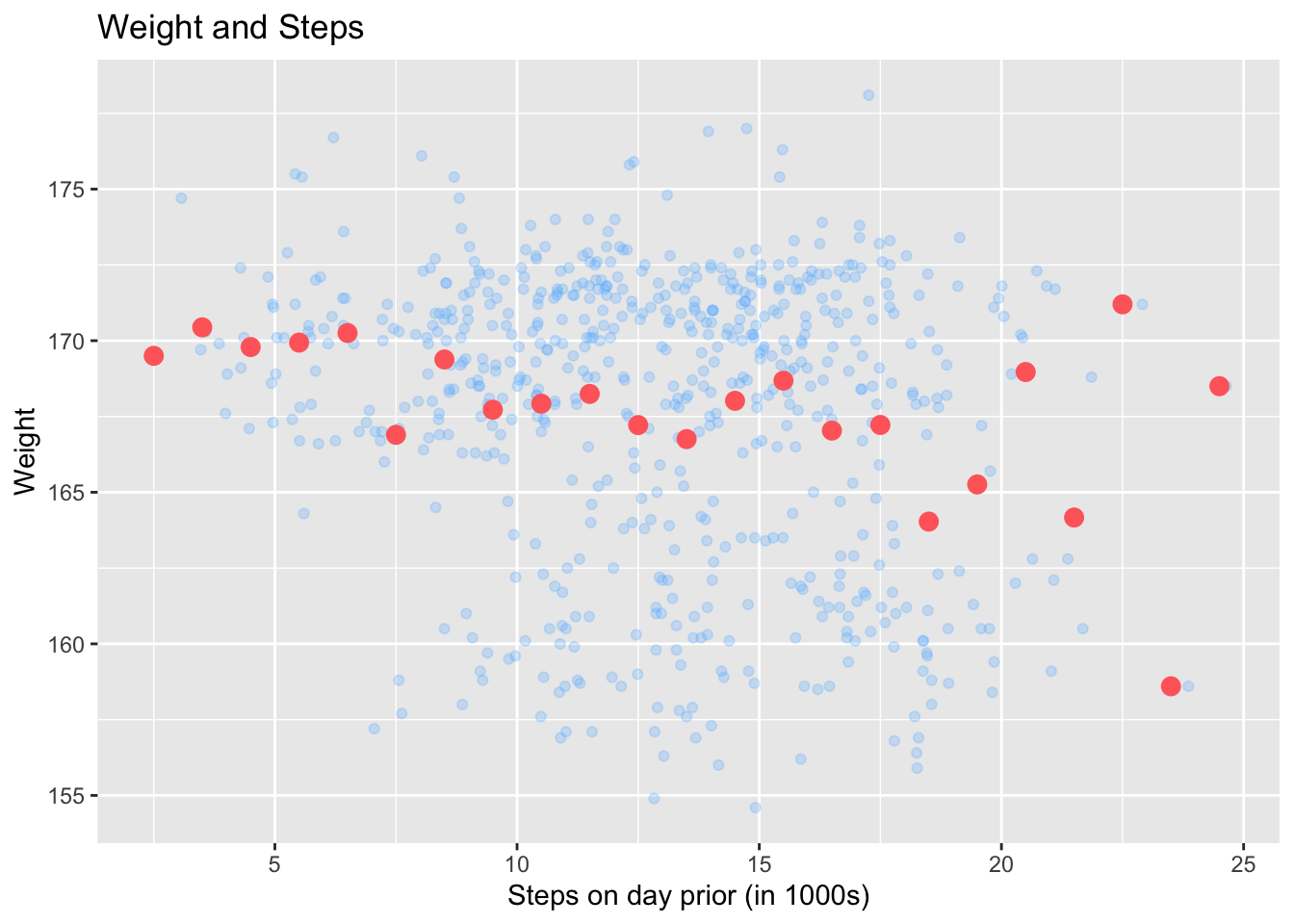
Running a regression (estimating the line of best fit)
We can estimate the line of best fit using the lm function:
fit <- lm(weight ~ steps, data = health)
fit
Call:
lm(formula = weight ~ steps, data = health)

Coefficients:
(Intercept)        steps
   170.5435      -0.2206
Extracting the vector of estimated regression coefficients
coef(fit)(Intercept) steps
170.5434834 -0.2205511 Obtaining unit-level statistics about the regression
The broom package has a number of functions that will allow you to extract information about the regression output from lm(). For example, if you want information about each unit such as the predicted/fitted value and the residual, you can use augment:
library(broom)
augment(fit)
# A tibble: 644 × 8
weight steps .fitted .resid .hat .sigma .cooksd .std.resid
<dbl> <dbl> <dbl> <dbl> <dbl> <dbl> <dbl> <dbl>
1 168 17.5 167. 1.31 0.00368 4.69 0.000146 0.281
2 169. 18.4 166. 2.62 0.00463 4.69 0.000730 0.560
3 168 19.6 166. 1.78 0.00609 4.69 0.000444 0.381
4 167. 10.4 168. -1.05 0.00217 4.69 0.0000547 -0.224
5 168. 18.7 166. 1.78 0.00496 4.69 0.000362 0.381
6 168. 9.14 169. -0.728 0.00296 4.69 0.0000359 -0.156
7 166. 8.69 169. -2.33 0.00331 4.69 0.000412 -0.498
8 168. 13.8 167. 0.911 0.00165 4.69 0.0000313 0.195
9 169 11.9 168. 1.08 0.00165 4.69 0.0000439 0.231
10 169. 24.6 165. 4.19 0.0155 4.68 0.00639 0.902
# ℹ 634 more rowsObtaining overall information about the model fitted
The glance function will give you some high-level information about the regression, including the \(R^2\):
glance(fit)# A tibble: 1 × 12
r.squared adj.r.squared sigma statistic p.value df logLik AIC BIC
<dbl> <dbl> <dbl> <dbl> <dbl> <dbl> <dbl> <dbl> <dbl>
1 0.0332 0.0317 4.68 22.1 0.00000323 1 -1907. 3820. 3834.
# ℹ 3 more variables: deviance <dbl>, df.residual <int>, nobs <int>You can also access the \(R^{2}\) using the summary() function:
summary(fit)$r.squared[1] 0.03322261Running a multiple regression
You can fit a regression with multiple predictors by putting a + between them on the right-hand side of the formula:
mult.fit <- lm(seat_change ~ approval + rdi_change,
               data = midterms)
mult.fit
Call:
lm(formula = seat_change ~ approval + rdi_change, data = midterms)

Coefficients:
(Intercept)     approval   rdi_change
   -117.226        1.526        3.217
Sampling (Week 9)
Selecting a random subset of rows of the data
The slice_sample function will return a random subset of rows from your data:
class_years |>
  slice_sample(n = 5)
# A tibble: 5 × 1
year
<chr>
1 Junior
2 Not Set
3 Sophomore
4 First-Year
5 First-YearRepeated sampling from a data frame
You can take multiple random samples from a data set using the rep_slice_sample function from the infer package. In the resulting data frame you will get a new column called replicate which will indicate which of the repeated samples this row belongs to.
library(infer)
class_years |>
  rep_slice_sample(n = 5, reps = 2)
# A tibble: 10 × 2
# Groups: replicate [2]
replicate year
<int> <chr>
1 1 First-Year
2 1 Junior
3 1 Graduate Year 1
4 1 Sophomore
5 1 Junior
6 2 Sophomore
7 2 First-Year
8 2 Sophomore
9 2 Sophomore
10 2 Junior You can use this to get repeated draws of a sample statistic like the sample proportion:
samples_n20 <- class_years |>
  rep_slice_sample(n = 20, reps = 100) |>
  group_by(replicate) |>
  summarize(fy_prop = mean(year == "First-Year"))
samples_n20
# A tibble: 100 × 2
replicate fy_prop
<int> <dbl>
1 1 0.35
2 2 0.3
3 3 0.5
4 4 0.3
5 5 0.3
6 6 0.3
7 7 0.4
8 8 0.2
9 9 0.15
10 10 0.3
# ℹ 90 more rowsConverting a column of a tibble into a vector
You can use the pull function to access a column of a tibble as a R vector, removing all the tibble infrastructure:
class_years |>
  slice_sample(n = 5) |>
  pull(year)
[1] "First-Year" "Sophomore" "Junior" "Junior" "Sophomore" Barplot with proportions rather than counts
You can use the y = after_stat(prop) aesthetic to get a barplot with proportions instead of count to show us the chance/probability of selecting a first-year student:
class_years |>
  mutate(first_year = as.numeric(year == "First-Year")) |>
  ggplot(aes(x = first_year)) +
  geom_bar(mapping = aes(y = after_stat(prop)), width = 0.1)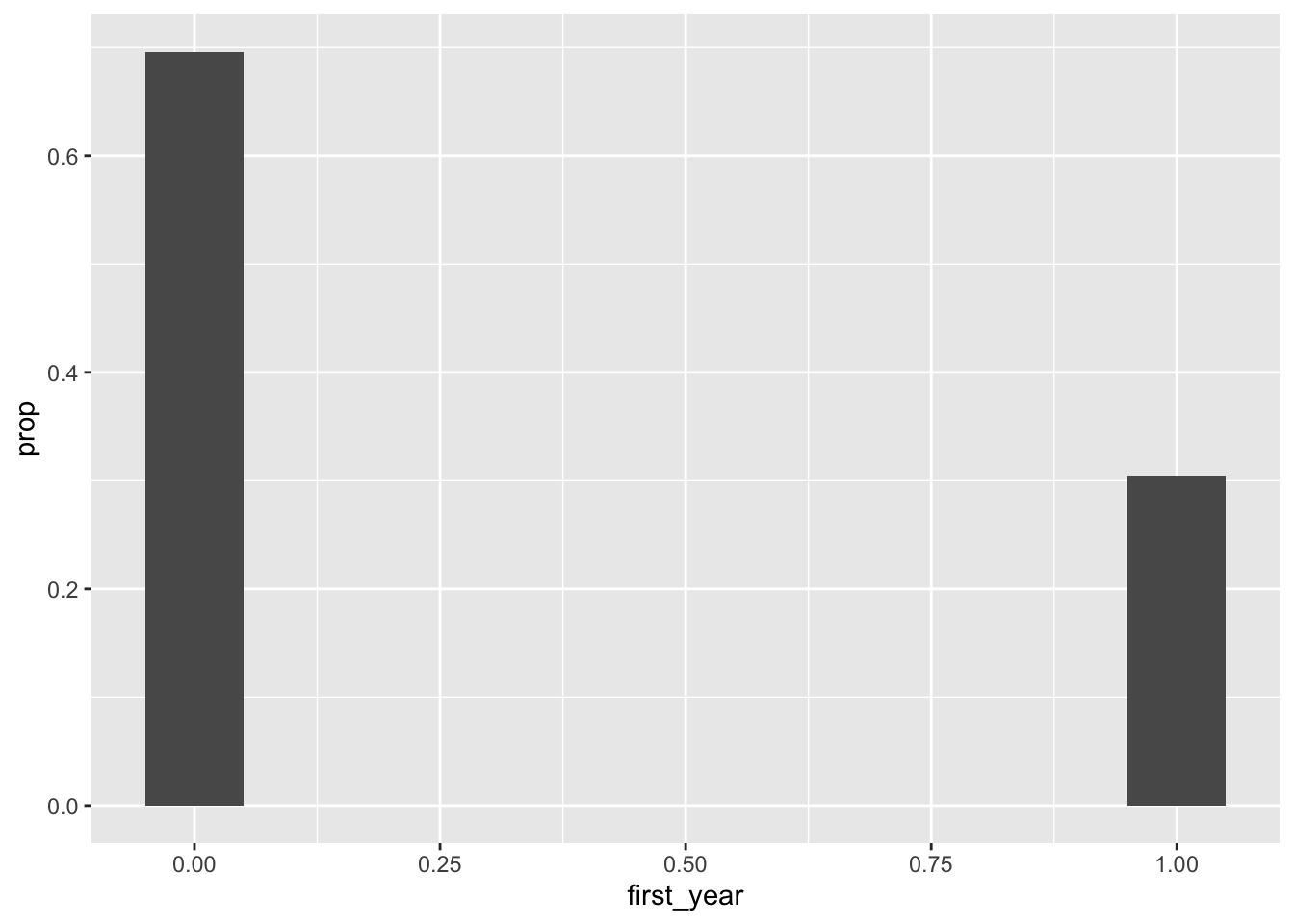
Density histograms
We can use the y = after_stat(density) to create a density histogram instead of a count histogram so that the area of the histogram boxes are equal to the chance of randomly selecting a unit in that bin:
midwest |>
  ggplot(aes(x = percollege)) +
  geom_histogram(aes(y = after_stat(density)), binwidth = 1)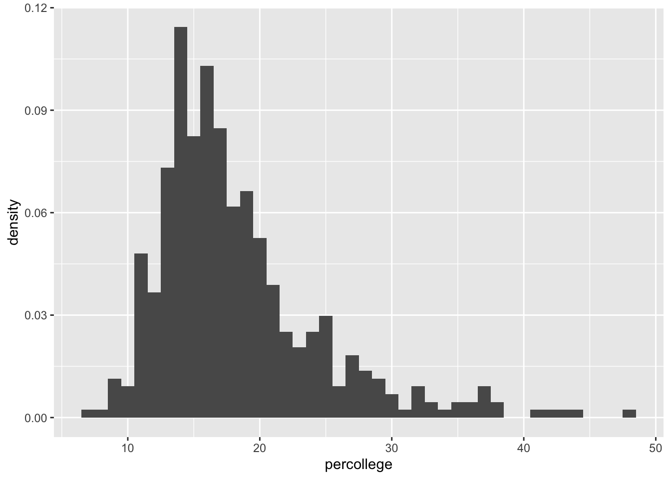
Bootstrap (Week 10)
Bootstrap distributions
You can generate bootstrap samples by using rep_slice_sample(prop = 1, replace = TRUE). From there, if you group by the replicate column, you can do summaries within each bootstrap sample.
bootstrap_dist <- anes |>
  rep_slice_sample(prop = 1, reps = 1000, replace = TRUE) |>
  group_by(replicate) |>
  summarize(sci_therm_mean = mean(sci_therm))
bootstrap_dist
# A tibble: 1,000 × 2
replicate sci_therm_mean
<int> <dbl>
1 1 80.6
2 2 80.8
3 3 80.3
4 4 80.8
5 5 80.4
6 6 80.6
7 7 80.4
8 8 80.7
9 9 80.8
10 10 80.5
# ℹ 990 more rowsYou can also generate bootstraps using the specify/generate workflow:
boot_dist_infer <- anes |>
  specify(response = sci_therm) |>
  generate(reps = 1000, type = "bootstrap") |>
  calculate(stat = "mean")
boot_dist_infer
Response: sci_therm (numeric)
# A tibble: 1,000 × 2
replicate stat
<int> <dbl>
1 1 80.6
2 2 80.7
3 3 80.9
4 4 80.9
5 5 80.7
6 6 80.6
7 7 80.5
8 8 80.7
9 9 80.3
10 10 80.6
# ℹ 990 more rowsYou can also pass these functions to visualize() to plot the distributions (though you could always use ggplot as well):
visualize(boot_dist_infer)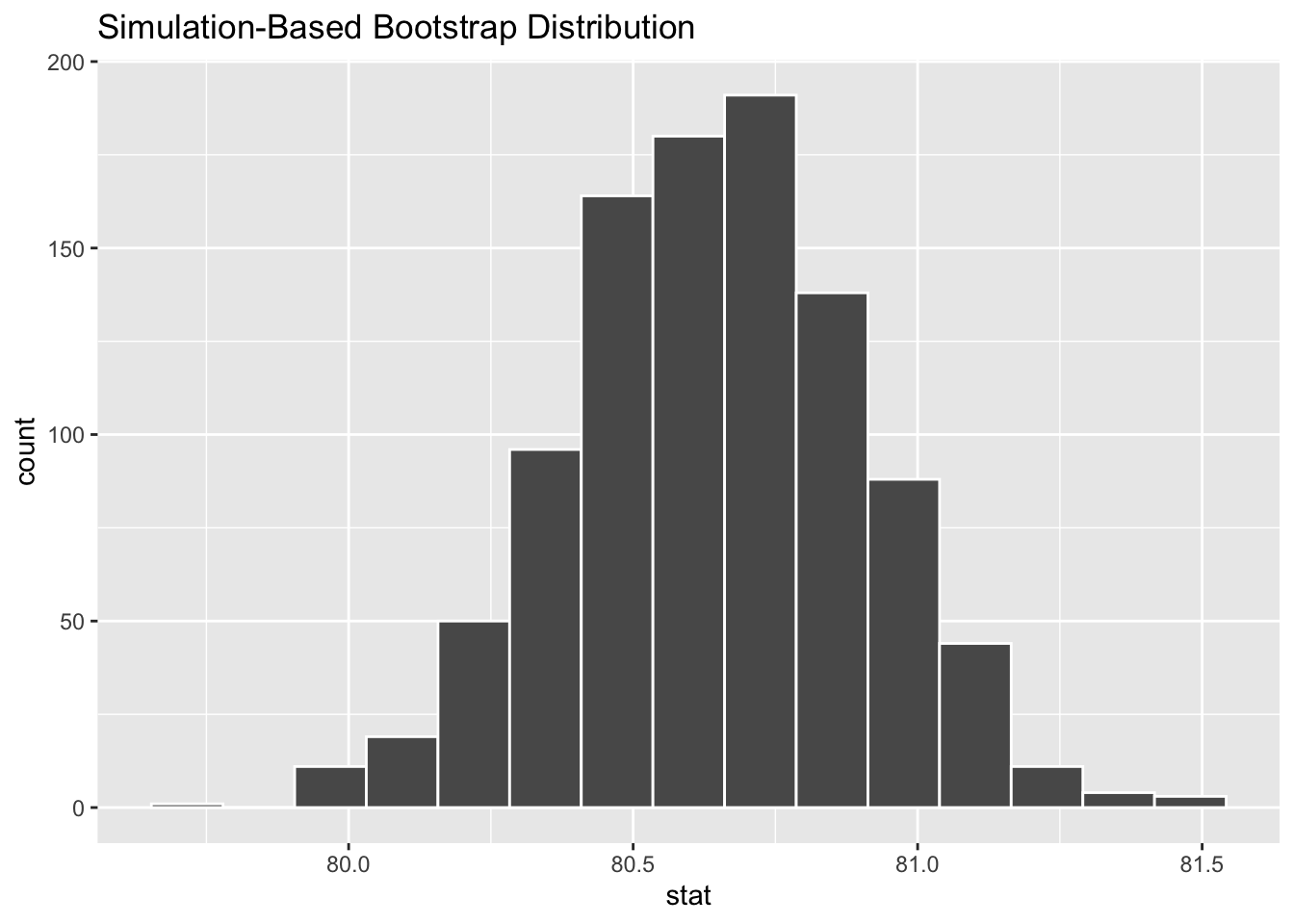
Calculating bootstrap confidence intervals
You can use the get_confidence_intervals or get_ci (they are the same function) with type = "percentile" to get bootstrap confidence intervals. Use the level argument to set the confidence level
boot_dist_infer |>
  get_confidence_interval(level = 0.95, type = "percentile")
# A tibble: 1 × 2
lower_ci upper_ci
<dbl> <dbl>
1 80.1 81.1Bootstrapping a difference in means
To get the bootstrapped distribution of a difference in means, we can use rep_slice_sample and our usual dplyr workflow:
dim_boots <- trains |>
  rep_slice_sample(prop = 1, replace = TRUE, reps = 1000) |>
  group_by(replicate, treatment) |>
  summarize(post_mean = mean(numberim.post)) |>
  pivot_wider(names_from = treatment, values_from = post_mean) |>
  mutate(ATE = `1` - `0`)
`summarise()` has grouped output by 'replicate'. You can override using the
`.groups` argument.dim_boots# A tibble: 1,000 × 4
# Groups: replicate [1,000]
replicate `0` `1` ATE
<int> <dbl> <dbl> <dbl>
1 1 2.65 3.04 0.395
2 2 2.80 3.20 0.399
3 3 2.62 2.95 0.327
4 4 2.71 2.88 0.172
5 5 2.71 2.98 0.263
6 6 2.70 3.04 0.344
7 7 2.95 3.13 0.182
8 8 2.78 3.30 0.522
9 9 2.71 3.24 0.532
10 10 2.87 3.26 0.388
# ℹ 990 more rowsNote that if you use this approach, you’ll need to select the column that you want before passing it to get_ci:
dim_boots |>
  select(replicate, ATE) |>
  get_ci(level = 0.95)
# A tibble: 1 × 2
lower_ci upper_ci
<dbl> <dbl>
1 0.0519 0.702We can also use the specify workflow from infer, but we need to be careful about setting the order of the groups for the difference in means in the calculate step:
dim_boots_infer <- trains |>
  mutate(treatment = if_else(treatment == 1, "Treated", "Control")) |>
  specify(numberim.post ~ treatment) |>
  generate(reps = 1000, type = "bootstrap") |>
  calculate(stat = "diff in means", order = c("Treated", "Control"))
dim_boots_infer
Response: numberim.post (numeric)
Explanatory: treatment (factor)
# A tibble: 1,000 × 2
replicate stat
<int> <dbl>
1 1 0.662
2 2 0.216
3 3 0.613
4 4 0.393
5 5 0.379
6 6 0.453
7 7 0.339
8 8 0.244
9 9 0.247
10 10 0.422
# ℹ 990 more rowsBootstrapping the difference between estimated ATEs
When you want to estimate the interaction between two variables or the difference in ATEs between two groups, we need to get both the treatment and grouping variables into the columns using pivot_wider. Passing both variables to the names_from argument will create columns based on each combination of the variables with a _ to separate the column names:
trains |>
mutate(
treatment = if_else(treatment == 1, "Treated", "Control"),
college = if_else(college == 1, "College", "Noncollege")
) |>
group_by(treatment, college) |>
summarize(post_mean = mean(numberim.post)) |>
pivot_wider(
names_from = c(treatment, college),
values_from = post_mean
) `summarise()` has grouped output by 'treatment'. You can override using the
`.groups` argument.# A tibble: 1 × 4
Control_College Control_Noncollege Treated_College Treated_Noncollege
<dbl> <dbl> <dbl> <dbl>
1 2.63 3.57 3.11 3.14Thus, to calculate the difference in ATEs we can:
trains |>
mutate(
treatment = if_else(treatment == 1, "Treated", "Control"),
college = if_else(college == 1, "College", "Noncollege")
) |>
group_by(treatment, college) |>
summarize(post_mean = mean(numberim.post)) |>
pivot_wider(
names_from = c(treatment, college),
values_from = post_mean
) |>
mutate(
ATE_c = Treated_College - Control_College,
ATE_nc = Treated_Noncollege - Control_Noncollege,
interaction = ATE_c - ATE_nc
)`summarise()` has grouped output by 'treatment'. You can override using the
`.groups` argument.# A tibble: 1 × 7
Control_College Control_Noncollege Treated_College Treated_Noncollege ATE_c
<dbl> <dbl> <dbl> <dbl> <dbl>
1 2.63 3.57 3.11 3.14 0.482
# ℹ 2 more variables: ATE_nc <dbl>, interaction <dbl>We can now add the rep_slice_sample step to produce a bootstrap distribution of this interaction:
int_boots <- trains |>
mutate(
treatment = if_else(treatment == 1, "Treated", "Control"),
college = if_else(college == 1, "College", "Noncollege")
) |>
rep_slice_sample(prop = 1, replace = TRUE, reps = 1000) |>
group_by(replicate, treatment, college) |>
summarize(post_mean = mean(numberim.post)) |>
pivot_wider(
names_from = c(treatment, college),
values_from = post_mean
) |>
mutate(
ATE_c = Treated_College - Control_College,
ATE_nc = Treated_Noncollege - Control_Noncollege,
interaction = ATE_c - ATE_nc
) |>
select(replicate, ATE_c, ATE_nc, interaction)`summarise()` has grouped output by 'replicate', 'treatment'. You can override
using the `.groups` argument.int_boots# A tibble: 1,000 × 4
# Groups: replicate [1,000]
replicate ATE_c ATE_nc interaction
<int> <dbl> <dbl> <dbl>
1 1 0.240 -0.667 0.907
2 2 0.647 -0.319 0.967
3 3 0.667 -0.857 1.52
4 4 0.284 0.375 -0.0908
5 5 0.358 0.25 0.108
6 6 0.428 0.667 -0.239
7 7 0.596 -0.667 1.26
8 8 0.444 -1.14 1.59
9 9 0.8 0.143 0.657
10 10 0.360 -0.321 0.682
# ℹ 990 more rowsHypothesis testing (Week 11)
Generating the null distribution of a sample mean
null_dist <- gss |>
specify(response = hours) |>
hypothesize(null = "point", mu = 40) |>
generate(reps = 1000, type = "bootstrap") |>
calculate(stat = "mean")
null_distResponse: hours (numeric)
Null Hypothesis: point
# A tibble: 1,000 × 2
replicate stat
<int> <dbl>
1 1 40.4
2 2 39.0
3 3 39.1
4 4 41.2
5 5 40.8
6 6 40.1
7 7 39.9
8 8 40.7
9 9 40.2
10 10 40.5
# ℹ 990 more rowsCalculating the p-value of a hypothesis test
If we want to calculate the p-value of the test, we need to first calculate the observed value of the sample mean and then pass that to the get_p_value function:
obs_mean <- gss |>
specify(response = hours) |>
calculate(stat = "mean")
get_p_value(null_dist, obs_mean, direction = "both")# A tibble: 1 × 1
p_value
<dbl>
1 0.038We can also visualize the p-value:
visualize(null_dist) +
shade_p_value(obs_mean, direction = "both")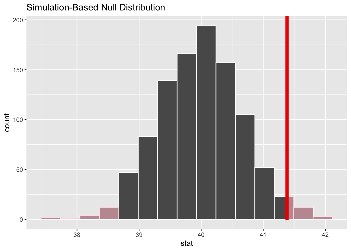
Null distribution for a difference in means
For a diffrence in means, we can use a similar approach, but need to turn our treatment/grouping variable into a charactor/factor variable. Then we need to make sure we sepcify the order the difference in mean should be taken across groups. First we calculate the effect and then get the null distribution using the permute approach.
trains <- trains |>
mutate(treated = if_else(treatment == 1, "Treated", "Untreated"))
ate <- trains |>
specify(numberim.post ~ treated) |>
calculate(stat = "diff in means",
order = c("Treated", "Untreated"))
ateResponse: numberim.post (numeric)
Explanatory: treated (factor)
# A tibble: 1 × 1
stat
<dbl>
1 0.383null_dist <- trains |>
specify(numberim.post ~ treated) |>
hypothesize(null = "independence") |>
generate(reps = 1000,
type = "permute") |>
calculate(stat = "diff in means", order = c("Treated", "Untreated"))
null_distResponse: numberim.post (numeric)
Explanatory: treated (factor)
Null Hypothesis: independence
# A tibble: 1,000 × 2
replicate stat
<int> <dbl>
1 1 -0.180
2 2 0.207
3 3 0.242
4 4 0.313
5 5 -0.0395
6 6 -0.145
7 7 -0.110
8 8 -0.0395
9 9 0.101
10 10 -0.110
# ℹ 990 more rowsGetting the p-value is the same:
get_p_value(null_dist, obs_stat = ate, direction = "both")# A tibble: 1 × 1
p_value
<dbl>
1 0.026